Bessel zero spacing

Bessel functions are to polar coordinates what sines and cosines are to rectangular coordinates. This is why Bessel function often arise in applications with radial symmetry.

The locations of the zeros of Bessel functions are important in application, and so you can find software for computing these zeros in mathematical libraries. In days gone by you could find them in printed tables, such as Table 9.5 in A&S.

Bessel functions are solutions to Bessel’s differential equation,

$x^2 y'' + x y' + (x^2 - \nu^2) y = 0$

For each ν the functions J_ν and Y_ν, known as the Bessel functions of the first and second kind respectively, form a basis for the solutions to Bessel’s equation. These functions are analogous to cosine and sine

As x → ∞, Bessel functions asymptotically behave like damped sinusoidal waves. Specifically,

$\begin{align*} J_\nu(x) &\sim \sqrt{\frac{2}{\pi x}} \cos(x - \pi\nu/2 - \pi/4) \\ Y_\nu(x) &\sim \sqrt{\frac{2}{\pi x}} \sin(x - \pi\nu/2 - \pi/4) \end{align*}$

So if for large x Bessel functions of order ν behave something like sin(x), you’d expect the spacing between the zeros of the Bessel functions to approach π, and this is indeed the case.

We can say more. If ν² > ¼ then the spacing between zeros decreases toward π, and if ν² < ¼ the spacing between zeros increases toward π. This is not just true of J_ν and Y_ν but also of their linear combinations, i.e. to any solution of Bessel’s equation with parameter ν.

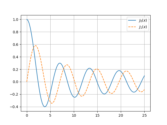
If you look carefully, you can see this in the plots of J₀ and J₁ below. The solid blue curve, the plot of J₀, crosses the x-axis at points closer together than π, and dashed orange curve, the plot of J₁, crosses the x-axis at points further apart than π.

For more on the spacing of Bessel zeros see [1].

[1] F. T. Metcalf and Milos Zlamal. On the Zeros of Solutions to Bessel’s Equation. The American Mathematical Monthly, Vol. 73, No. 7, pp. 746–749

Bessel zero spacing

Related posts

Leave a Reply