
Common sense says that what you believe after seeing new data should be some sort of compromise between what you believed before and what the new data says. You don’t want to ignore previous information or new information.
How much should new data change your prior beliefs? When prior judgment and new information are in conflict, which one should be given the benefit of the doubt?
Bayesian data models provide a framework for making such decisions quantitative and objective. The choice of a data model is somewhat subjective—whether it’s a Bayesian model or not—but given a Bayesian model, the rules for updating the representation of your beliefs are objective. As some put it, you “turn the Bayesian crank.” A likelihood model and a prior on parameters together specify how new data changes the prior distribution into a posterior distribution.
We will make this more concrete with three examples.
Normal-normal model
Suppose that data X has a normal distribution with unknown mean μ and known variance σ², and we assume that a priori μ has a normal distribution with mean μ0 and variance σ0².
After observing x, the posterior distribution on μ also has a normal distribution, but with a different mean and variance. Its mean is somewhere between the prior mean and x. We will ignore the change in the variance for this post.
The posterior mean of μ is
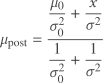
This equation becomes more understandable when we introduce precisions τ = 1/σ² and τ0 = 1/σ0².
Then we have
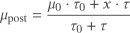
which you can read as saying the posterior mean is the weighted average of the prior mean and x, with the weights given by the precision. Intuitively, you take the weighted mean of your conclusions from previous data and new data, weighting the mean according to how much confidence you have in each.
Beta-binomial model
Now let’s switch over to a different data model. Now assume X is a binary random variable, with probability of success p and probability of failure 1 − p, and we assume p has a beta(a, b) distribution.
After observing s successes and f failures, the posterior mean of the distribution on p becomes
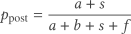
We can rewrite this as
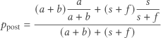
This says that the posterior mean is the weighted average of the prior mean a/(a + b) and the mean of the data s/n. The weights are the prior effective sample size a + b and the sample size of the new data n. In this example (effective) sample size is playing the role that precision played in the normal-normal model above.
Gamma-Poisson model
Suppose data have a Poisson distribution with parameter λ, and λ has a gamma(α0, β0) prior distribution [1]. And suppose you observe k events over time t. Then the posterior distribution of λ given the data has a gamma(α0 + k, β0 + t) prior distribution and the mean of the posterior distribution is given by

As before, the posterior mean is a weighted average of the prior mean and new data, and the weights are interpretable as some sort of measure of confidence, namely time. The variable t is directly time and the parameter β0 is sort of an effective time, just as a + b is an effective sample size for the beta distribution.
Common thread
In each example the posterior mean is the weighted average of the prior mean and the mean of the data, with the weights given by a precision. However, precision means something different in each example. In the normal-normal model, precision is the reciprocal of variance, but in the beta-binomial model precision is sample size and in the Poisson-gamma model precision is time.
What all three examples have in common is that they are conjugate models using distributions from the “exponential family” of probability distributions. In technical terms, precision is the multiplicative factor on the sufficient statistic in the exponent of the posterior kernel.
Related posts
- Does additional data always reduce posterior variance?
- Diagram of probability distribution relationships
- Bayesian statistics consulting
[1] There are multiple conventions for parameterizing the gamma distribution. Here we’re using the shape-rate parameterization, where the mean is α/β.