Golden integration

Let φ be the golden ratio. The fractional parts of nφ bounce around in the unit interval in a sort of random way. Technically, the sequence is quasi-random.

Quasi-random sequences are like random sequences but better in the sense that they explore a space more efficiently than random sequences. For this reason, Monte Carlo integration (“integration by darts“) can often be made more efficient by replacing random sequences with quasi-random sequence. This post will illustrate this efficiency advantage in one dimension using the fractional parts of nφ.

Here are functions that will generate our integration points.

    from numpy import random, zeros

    def golden_source(n):
        phi = (1 + 5**0.5)/2
        return (phi*n)%1

    def random_source(N):
        return random.random()

We will pass both of these generators as arguments to the following function which saves a running average of function evaluates at the generated points.

    def integrator(f, source, N):
        runs = zeros(N)
        runs[0] = f(source(0))
        for n in range(1, N):
            runs[n] = runs[n-1] + (f(source(n)) - runs[n-1])/n
        return runs

We’ll use as our example integrand f(x) = x² (1 – x)³. The integral of this function over the unit interval is 1/60.

    def f(x):
        return x**2 * (1-x)**3
    exact = 1/60

Now we call our integrator.

    random.seed(20230429)
    N = 1000
    golden_run = integrator(f, golden_source, N)
    random_run = integrator(f, random_source, N)

Now we plot the difference between each run and the exact value of the integral. Both methods start out with wild fluctuations. We leave out the first 10 elements in order to make the error easier to see.

    import matplotlib.pyplot as plt

    k = 10
    x = range(N)
    plt.plot(x[k:], golden_run[k:] - exact)
    plt.plot(x[k:], random_run[k:] - exact)

This produces the following plot.

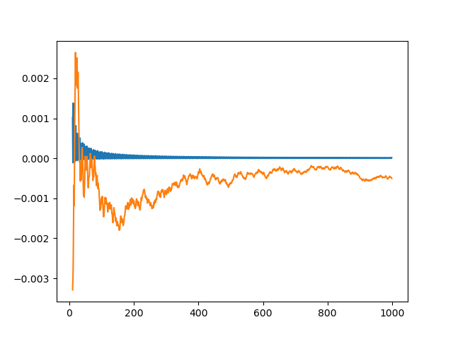
The integration error using φn – ⌊φn⌋ is so close to zero that it’s hard to observe its progress. So we plot it again, this time taking the absolute value of the integration error and plotting on a log scale.

    plt.plot(x[k:], abs(golden_run[k:] - exact))
    plt.plot(x[k:], abs(random_run[k:] - exact))
    plt.yscale("log")

This produces a more informative plot.

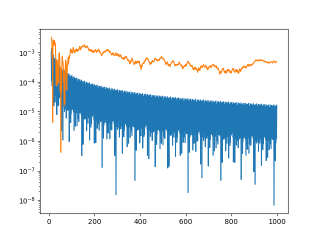
The integration error for the golden sequence is at least an order of magnitude smaller, and often a few orders of magnitude smaller.

The function we’ve integrated has a couple features that make integration using quasi-random sequences (QMC, quasi-Monte Carlo) more efficient. First, it’s smooth. If the integrand is jagged, QMC has no advantage over MC. Second, our integrand could be extended smoothly to a periodic function, i.e. f(0) = f(1) and f′(0) = f′(1). This makes QMC integration even more efficient.

Related posts

• Intro to QMC and discrepancy
• Quality of an RNG depends on the application
• QMC for periodic and nonperiodic functions