
I’ve written three posts on cosine similarity lately. The first looked at interpreting cosine similarity. The second looked at an approximation related to the first. The third looked at how ranking according to cosine similarity works better than cosine similarity itself.
Normalized word vectors are points on a high dimensional sphere, and geometry in high dimensions is counterintuitive. See the first post in this series for an explanation.
The set of points within a given angular distance of a point on a hypersphere is called a spherical cap. The ratio of the area of this spherical cap to that of the whole sphere is called cap fraction or concentration ratio. Concentration ratio explains why a modest cosine similarity value corresponds to a tiny portion of the area of the sphere and should be interpreted as a close match.
For this post, I wanted to share a plot of concentration ratio as a function of cosine similarity.
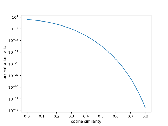
This shows that moderate values of cosine similarity correspond to infinitesimal concentration ratios. And yet, as the third post linked at the top showed, word vectors are very unevenly distributed, and even extremely small regions of the sphere can contain multiple word vectors.
I only included cosine similarity values up to 0.8 because the function plotted above takes a nosedive for larger values, even on a logarithmic scale.
Here’s the Python code to make the plot, using the function cap_fraction from here.
s = np.linspace(0, 0.8, 500)
plt.plot(s, cap_fraction(np.acos(s), 200))
plt.yscale("log")
plt.xlabel("cosine similarity")
plt.ylabel("concentration ratio")
plt.show()