Looking at Your Data

What to do first after scoping out and starting a data science project?

I’ve started an unsupervised learning project based on textual data. The first thing I like to do is actually look at the data. Is it noisy? What are the features—complex feature engineering needed? How heterogeneous? What generalization and overfitting challenges?

Analysis can take many forms: actually looking at the numbers, using visualization tools, Excel spreadsheet, Jupyter notebooks with Matplotlib, computing various statistics on the whole dataset or portions of it.

Some may believe this is not important. Just throw a barrage of classification or regression methods at the data, treat the data as a black box. Of course testing on a suite of ML methods is not a bad thing. But I can’t imagine not using every avenue available, including looking at the data. I’m certainly not alone in this view (see for example herehere and here).

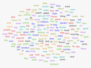
I spent a few hours developing a simple custom data viewer for my problem that colored different parts of the textual data to give insight as to what was going on. I used ChatGPT to develop parts of this tool; some of it was incorrect and needed fixing, but having at least a draft of the code definitely saved time. Seeing the actual data in person was insightful and generated ideas for solving the problem.

While inspecting the data can help identify issues, it also risks biasing the modeling process by imposing assumptions that a flexible model might otherwise uncover on its own. One must also beware of data leakage. That being said—in general I think understanding as much as you can about the data is not a bad thing.

Lessons Learned With the Z3 SAT/SMT Solver

Community best practices are useful for helping use a software product more effectively. I’ve just completed a small project using the Z3 solver. Here are some things I’ve learned:

  • My project involves an optimization problem: for a subset of Boolean variables, maximize the count of how many are true. My specific problem is solved much faster with Z3 by converting to a decision problem: set up a base problem to solve for the count being at least a certain fixed number, and iterate using bisection search to find the highest number satisfied. Bisection has been used for this problem before. Also, certain methods may possibly reduce the number of bisection steps.
  • Using Z3  “tactics” can greatly speed up the solve process. I found a good combination of tactics by trial and error, guided in part by the descriptions of the tactics. ChatGPT was of some help in finding good selections to try. An interesting paper discusses use of Monte Carlo tree search to define a good chain of tactics. The branching factor here is high, perhaps around 1000, though there are some redundancies in this number. Training multi-step MCTS might be expensive, but doing this once to get a good static chain of tactics might be worthwhile.
  • The strength of Z3 is in its extremely broad functionality, more so than its raw compute performance. It would be a daunting task for the Z3 team to fully optimize every possible solve option. I examined some of the SMT solver competitions to find faster codes. CVC5 on one case I tried was about twice as fast as Z3; I’ve seen similar reports in the literature. Presently I don’t find it worth the switching costs to use CVC5. One approach might be to use the very capable tactics engine of Z3 and pass the resulting modified problem to CVC5.
  • The specific formulation of the problem can make a big difference in solver performance. I’ve already seen this in the area of iterative linear solvers, for example diagonal matrix scaling can dramatically help (conjugate gradients) or hurt (multigrid) solver performance. Same thing here. Hence the huge importance in good “preprocessing“ for SAT/SMT solvers. One could wish the solver could handle all this automatically without user intervention. However, these powerful tools must be brandished very carefully for maximum effect.
  • Generally, one should move as much of the problem outside of the solver as possible, since the solver is the long pole in the tent in terms of scalability. For example if there is a Z3 integer that must be limited to a certain range and additionally some values in the interval must be blacklisted, it’s better, if possible, to compress all of the valid values into a single interval, to make testing for validity simpler in the Z3 code.
  • Along these lines: the Z3 tactics for propagating constants are not perfect; thus it can help to manually propagate constants (though this unfortunately makes the code more messy). This propagation can also sometimes allow for removal of unneeded constraints, further speeding up performance. Relatedly, some intriguing work by Benjamin Mikek shows how one can use the LLVM code optimizer to optimize the SMT problem in a way that is complementary to Z3 tactics, achieving significant speedup (for more info see here, here and here). I haven’t tried this but it seems promising.
  • Because of the scalability challenge of SMT solvers, various simplifying heuristics to modify the problem can be helpful. For example: solving a subproblem of the main problem and holding the resulting variables fixed in order to solve the rest of the problem. Or solving a simpler, smaller problem first to determine variable presets for the full problem. With these heuristics, one does not in general find the true global optimum; but the result may be adequate.
  • CPU threading does not work for my case (Z3 Python, macOS). Perfect parallelization of SAT and SMP is an unsolved (and perhaps in some sense not fully solvable) problem. One can naïvely parallelize bisection search by converting to trisection, etc., but this does not give perfect speedup (specif., log(P) speedup on P threads). Improvements to parallel bisection in some cases may be possible. Recent work by Armin Biere and colleagues looks promising; as I read it, near perfect speedup up to eight threads (at least for some problems).
  • Some of the main developers of Z3 are on Stack Overflow and have been active in the past answering questions. This seems very useful.

Resources like Handbook of Satisfiability and the proceedings of various SAT/SMT conferences seem helpful. More information on best practices for non-expert practitioners would be a great help to the community. If you know of any good resources, please share in the comments.

DeepSeek-R1: Do we need less compute now?


The reactions to the new DeepSeek-R1 AI model in recent days seem limitless. Some say it runs so much faster than existing models that we will no longer need the billions of dollars in compute hardware that big tech is preparing to buy.

Is that plausible?

To get an answer, we need only look back at the experience of the recently-completed Exascale Computing Project. This large scale multi-lab project was tasked with developing technology (primarily software) to prepare for exascale computing, which has recently been achieved by Frontier, Aurora and El Capitan.

During the course of the project, various algorithm and implementation improvements were discovered by the the science teams, these leading to as much as 60X speedup or more, over and above speedups possible from hardware alone [1]. In response, are the teams just running the very same problems faster on older hardware? No — instead, they are now able to run much, much larger problems than previously possible, exploiting both hardware and software improvements.

Or suppose today there were no such thing as the fast Fourier transform (FFT) and scientists were computing Fourier transforms using (essentially) large dense matrix-vector products. If someone then discovered the FFT, I’d guarantee you that scientists would not only say, (1) “Wow, now I can run my existing problems much, much faster,” but also, (2) “Wow, now I can run problems much larger than I ever dreamed and solve problems larger than I could have ever imagined!”

Paradoxically, faster algorithms might even increase the demand for newer, faster hardware. For example, a new faster algorithm for designing medications to cure cancer might be judged so important that it’s worth building the largest machine possible to run it effectively.

All this is not to say whether you should buy or sell Nvidia stock right now. However, it does mean that there is no simplistic argument that faster algorithms and implementations necessarily lead to lower spend on computing hardware. History shows that sometimes this is not true at all. The smart money, on the other hand, is on research teams that are able to exploit any and every new discovery to improve what is possible with their codes, whether by hardware, data, code optimizations or algorithms.

Notes

[1] See slide 9 from Doug Kothe’s talk, “Exascale and Artificial Intelligence: A Great Marriage“. The “Figure of Merit” (FOM) number represents speedup of science output from an application compared to an earlier baseline system. Specifically, a FOM speedup of 50X is the anticipated speedup from baseline due to efficient use of hardware only, for example, on Frontier compared to the earlier OLCF Titan system.

Can AI models reason like a human?

We’re awaiting the release of OpenAI’s o3 model later this month. Its performance is impressive on very hard benchmarks like SWE-bench Verified, Frontier Math and the ARC AGI benchmark (discussed previously in this blog).

And yet at the same time some behaviors of the frontier AI models are very concerning.

Their performance on assorted math exams is outstanding, but they make mistakes doing simple arithmetic, like wrongly multiplying numbers that are a few digits long. Performance of the o1 preview model on the difficult Putnam math exam is excellent but drops precipitously under simple changes like renaming constants and variables in the problem statement.

Similarly, when o1 is applied to a planning benchmark expressed in standardized language, it performs well, but accuracy falls apart when applied to a mathematically equivalent planning problem in a different domain. And also, a given AI model applied to the simple ROT13 cipher can have wildly different performance based on the value of the cipher key, suggesting the models don’t really understand the algorithm.

It was the best of times, it was the worst of times, . . .

What is going on here?

For years now, some have made claims of “human-level performance” for various deep learning algorithms. And as soon as one party starts making claims like this, it’s hard for the others to resist doing the same.

The confusion is that, from a certain point of view, the claim of “human-level” is true—but the definition of “human-level” is fraught.

Here, “human-level” is taken to mean achievement of some high score on a benchmark set, ostensibly exceeding some human performance measure on the same benchmark. However, a single AI model can vary wildly in capability across behaviors—“smart” compared to humans in some ways, “dumb” in others.

For humans, test-taking is a proxy for measuring a range of skills and abilities. And even for humans it is not always an accurate proxy. A person can perform very well on academic tests and very poorly on the job, or vice versa.

And the capability ratios for AI models are very different still, in ways we don’t fully understand. So, outscoring humans on a software engineering benchmark doesn’t mean the AI has the whole panoply of coding skills, decision-making abilities, software architecture design savvy, etc., needed to be a competent software engineer.

It’s no surprise that recent articles (below) show a growing perception of the limitations of AI benchmarks as currently conceived.

Ways forward

Perhaps we should consider developing requirements like the following before claiming human-level reasoning performance of an AI model:

  • It should be able to “explain its work” at any level of detail to another human (just like a human can), in a way that that human can understand.
  • It should be able to give answers without “hallucinating” or “confabulating” (yes, humans can hallucinate too, but most occupations would not be well-served by an employee who hallucinates on the job).
  • It should be able to reliably and consistently (100% of the time) do things that we routinely expect a human or computer to do accurately (like add or multiply two numbers accurately, for things like filling out tax returns or doing engineering calculations to build an airplane).
  • It should be frank and honest in assessing its level of certainty about an answer it gives (no gaslighting).
  • It should be able to solve a trivial perturbation of a given problem with the same ease as the original problem (to the same extent that a human can).
  • As someone has said, it should be able to do, without specific training, what a 5 year old can do without specific training.
  • This one sounds good, from Emmett Shear: “AGI [artificial general intelligence] is the ability to generalize [without special training by a human] to an adversarially chosen new benchmark.”

AI models are fantastic and amazing tools—and best used when one has eyes wide open about their limitations.

Have you had problems with AI model performance? If so, please share in the comments.

References

Rethinking AI benchmarks: A new paper challenges the status quo of evaluating artificial intelligence, https://venturebeat.com/ai/rethinking-ai-benchmarks-a-new-paper-challenges-the-status-quo-of-evaluating-artificial-intelligence/

Rethink reporting of evaluation results in AI, https://www.science.org/doi/10.1126/science.adf6369, https://eprints.whiterose.ac.uk/198211/

Inadequacies of Large Language Model Benchmarks in the Era of Generative Artificial Intelligence, https://arxiv.org/abs/2402.09880

Everyone Is Judging AI by These Tests. But Experts Say They’re Close to Meaningless, https://themarkup.org/artificial-intelligence/2024/07/17/everyone-is-judging-ai-by-these-tests-but-experts-say-theyre-close-to-meaningless

Why we must rethink AI benchmarks, https://bdtechtalks.com/2021/12/06/ai-benchmarks-limitations/

AI and the Everything in the Whole Wide World Benchmark, https://arxiv.org/abs/2111.15366

BetterBench: Assessing AI Benchmarks, Uncovering Issues, and Establishing Best Practices, https://arxiv.org/abs/2411.12990

Goodhart’s Law states that when a proxy for some value becomes the target of optimization pressure, the proxy will cease to be a good proxy.

Can AI models reason: Just a stochastic parrot?

OpenAI has just released its full o1 model—a new kind of model that is more capable of multi-step reasoning than previous models. Anthropic, Google and others are no doubt working on similar products. At the same time, it’s hotly debated in many quarters whether AI models actually “reason” in a way similar to humans.

Emily Bender and her colleagues famously described large language models as nothing more than “stochastic parrots“—systems that simply repeat their training data blindly, based on a statistical model, with no real understanding (reminiscent of the Chinese Room experiment). Others have made similar comments, describing LLMs as “n-gram models on steroids” or a “fancy extrapolation algorithm.

There is of course some truth to this. AI models sometimes generate remarkable results and yet lack certain basic aspects of understanding that might inhibit their sometimes generation of nonsensical results. More to the point of “parroting” the training data, recent work from Yejin Choi’s group has shown how LLMs at times will cut and paste snippets from its various training documents, almost verbatim, to formulate its outputs.

Are LLMs (just) glorified information retrieval tools?

The implication of these concerns is that an LLM can “only” repeat back what it was taught (albeit with errors). However this view does not align with the evidence. LLM training is a compression process in which new connections between pieces of information are formed that were not present in the original data. This is evidenced both mathematically and anecdotally. In my own experience, I’ve gotten valid answers to such obscure and detailed technical question that it is hard for me to believe would exist in any training data in exactly that form. Whether you would call this “reasoning” or not might be open to debate, but regardless of what you call it, it is something more than just unadorned information retrieval like a “stochastic parrot.”

What is your experience? Let us know in the comments.

The impossible puzzle

It’s fascinating that there’s such a thing as the World Jigsaw Puzzle Championship. The winning team of the two-person thousand-piece puzzle round can assemble a Ravensburger puzzle in less than an hour—that’s about 3 -1/2 seconds per piece.

It makes you wonder, how could you measure the hardness of a jigsaw puzzle? And what would a “hardest puzzle” look like?

You can find some puzzles that are claimed to be “hardest.” A first step to creating a hard puzzle is removing the front image entirely, eliminating visual cues. Some puzzles do this. This can be partly simulated with a normal puzzle by putting it together with the image side face down.

But you can do more: make every piece a square exactly the same size, and the “tab“ and “blank“ on each of the four sides of each square exactly the same size, shape and alignment. One can see that this gives you 24 = 16 different unique kinds of puzzle piece, however, due to symmetries you actually have six different kinds of puzzle piece. Now, you are left with a bare minimum of shape cues to help you assemble the puzzle.

For the sake of the argument, one can ignore the “edge” pieces. One can see this from the fact that for a rectangular puzzle, as you scale up the size, the number of edge pieces proportional to the interior pieces of the puzzle becomes smaller and smaller. For example for a 36X28=1008 piece puzzle, there are (2*36+2*28-4)=124 edge pieces, about 12 percent of the whole. The ratio shrinks as you scale up puzzle size. And there is such a thing as a 42,000-piece jigsaw puzzle.

The solution complexity class for assembling such a puzzle is known to be NP-complete. This means that the best known algorithms require compute time that grows exponentially as the number of pieces is increased.

Of course there are simpler special cases. Consider a checkerboard configuration, in which “black square“ location pieces have four tabs and “red square” locations have four blanks, thus only two different kinds of piece. A competent puzzler could assemble this one piece per second, 17 minutes for a 1000-piece puzzle.

However, as far as we know, the number of “special cases” like this is vanishing small for large puzzles. An intuition for this can be taken from Kolmogorov complexity theory, using a counting argument to show that only very few long strings can be compressed to a short program.

Most cases are really hard, for example, constructed by making a totally random assignment for selecting the configuration of each piece-to-piece boundary. Solving this is really hard because you may have to backtrack: you may have the puzzle largely complete, but due to ambiguities, you may need to backtrack because of a wrong decision made early.

A very weak upper bound in the assembly time can be derived by considering the brute force case. For a 1000-piece puzzle, there are 1000! (factorial) possible ways to (attempt to) assemble the puzzle. Suppose one places every piece and then fully backtracks for each trial—this gives 1000 x 1000! puzzle piece placement steps. Using Stirling’s approximation, this is approximately 104468 placement steps.

A human, assuming generously a rate of one step per second, at 31 million seconds/year nonstop, would take on the order of 104460 years. Assuming 10 billion simultaneous puzzlers—order 104450 years.

Now assume the on-record world’s fastest computer, the ORNL Frontier system (though see here), roughly 10 exaflops (1019) mixed precision, and assuming one puzzle step per operation (overly optimistic). Assume further that every atom in the known universe (est. 1082) is a Frontier computer system. In this case—solving the puzzle takes order 104359 years. That’s a thousand billion billion … (repeat “billion” 484 times here) years.

As I mentioned, this is a very weak upper bound. One could solve the problem using a SAT solver with sophisticated CDCL backtracking. Or one could use special methods derived from statistical mechanics that handle random SAT instances. However, to the best of our knowledge, the runtime still grows exponentially as a function of puzzle size. The best worst-case computational complexity for SAT solvers currently known is order O(1.306995n) (see here, here, and here). So, simply by constructing puzzles in the way we’ve described with more and more pieces, you will soon reach a point of having a puzzle that is unfathomably difficult to solve.

It’s conceivable that a yet-undiscovered method could be found for which the solution cost would in fact grow polynomially instead of exponentially. But people have been trying to answer this question one way or the other for over 50 years and it’s still unsolved, with an open million dollar prize for proof or counterexample. So we just don’t know.

What about quantum computing? It can solve some exponential complexity problems like factoring in polynomial time. But how about the SAT problem? It is simply not known (see here, here) whether a polynomial-time quantum algorithm exists for arbitrary NP-complete problems. None are known, and it might not be possible at all (though research continues).

So we’re faced with the curious possibility: a jigsaw puzzle could be constructed for which, you’re holding the box of pieces in your hand, you spill it on the floor, and there is no single or joint intelligence or computational mechanism, existing or even possible, in the entire universe that could ever reassemble it.

How hard is constraint programming?

I’ve been writing code for the Z3 SMT solver for several months now. Here are my findings.

Python is used here as the base language. Python/Z3 feels like a two-layer programming model—declarative code for Z3, imperative code for Python. In this it seems reminiscent of C++/CUDA programming for NVIDIA GPUs—in that case, mixed CPU and GPU imperative code. Either case is a clever combination of methodologies that is surprisingly fluent and versatile, albeit not a perfect blend of seamless conceptual cohesion.

Other comparisons:

  • Both have two separate memory spaces (CUDA CPU/GPU memories for one; pure Python variables and Z3 variables for the other).
  • Both can be tricky to debug. In earlier days, CUDA had no debugger, so one had to fall back to the trusty “printf” statement (for a while it didn’t even have that!). If the code crashed, you might get no output at all. To my knowledge, Z3 has no dedicated debugger. If the problem being solved comes back as satisfiable, you can print out the discovered model variables, but if satisfiability fails, you get very little information. Like some other novel platforms, something of a “black box.”
  • In both cases, programmer productivity can be well-served by developing custom abstractions. I developed a Python class to manage multidimensional arrays of Z3 variables, this was a huge time saver.

There are differences too, of course.

  • In Python, “=” is assignment, but in Z3, one only has “==”, logical or numeric equality, not assignment per se. Variables are set once and can’t be changed—sort of a “write-once variables” programming model—as is natural to logic programming.
  • Code speed optimization is challenging. Code modifications for Z3 constraints/variables can have extreme and unpredictable runtime effects, so it’s hard to optimize. Z3 is solving an NP-complete problem after all, so runtimes can theoretically increase massively. Speedups can be massive also; one round of changes I made gave 2000X speedup on a test problem. Runtime of CUDA code can be unpredictable to a lesser degree, depending on the PTX and SASS code generation phases and the aggressive code optimizations of the CUDA compiler. However, it seems easier to “see through” CUDA code, down to the metal, to understand expected performance, at least for smaller code fragments. The Z3 solver can output statistics of the solve, but these are hard to actionably interpret for a non-expert.
  • Z3 provides many, many algorithmic tuning parameters (“tactics”), though it’s hard to reason about which ones to pick. Autotuners like FastSMT might help. Also there have been some efforts to develop tools to visualize the solve process, this might be of help.

It would be great to see more modern tooling support and development of community best practices to help support Z3 code developers.

Preprocessing text to make it more compressible

Repetitive text compresses efficiently. Text like the lyrics to Jingle Bells ought to compress more efficiently than ordinary prose, assuming the compression algorithm can exploit the repetition.

The idea of the Burrows-Wheeler transform is to permute text in before compressing it. The hope is that the permutation will make the repetition in the text easier for a compression algorithm to take advantage of. The permutation must be reversible, so the compressed file can be uncompressed later.

It’s not immediately obvious that the Burrows-Wheeler transform is reversible; that may be the topic of another post some day. This post will explain what the transform is and show that it rearranges text in a way that makes run-length encoding more efficient.

Algorithm and example

The Burrows-Wheeler transform (BWT) lists all the rotations of a string in a table, sorts the table, then takes the last column as the transform value. (Software implementing the BWT does not need to actually construct the table, but it gives the same result as if it did.)

Before tabulating the rotations, the algorithm adds a character for beginning of string and one for end of string. We’ll use ^ and $ respectively, based on the meaning of these symbols in regular expressions.

Here is an example applied to wabisabi.

^wabisabi$          ^wabisabi$
$^wabisabi          $^wabisabi
i$^wabisab          abi$^wabis
bi$^wabisa          abisabi$^w
abi$^wabis          bi$^wabisa
sabi$^wabi          bisabi$^wa
isabi$^wab          i$^wabisab
bisabi$^wa          isabi$^wab
abisabi$^w          sabi$^wabi
wabisabi$^          wabisabi$^

The table on the left lists all rotations of ^wabisabi$, and the table on the right is the sorted form of the table on the left. The last column, $iswaabbi^, is the BWT of wabisabi. Note that the a‘s and the b‘s are grouped together in the transformed string.

When we sort the table we run into an annoying complication: what is the sort order of the markers for beginning of text and end of text? I used the Python code from the Wikipedia article on BWT for the examples below, so I followed the code’s sorting convention that the begin string symbol comes first, then the end string symbol, then ordinary text.

Run-length encoding

At the top of the post I mentioned the lyrics to Jingle Bells as an example of text with repetition. If we calculate the BTW of

jingle bells, jingle bells, jingle all the way.

we get

$.eee,,lessy w  lllhbbnnntjjj  ^lgggaeelliiill  a

Now we have a lot of repeated letters, which means we could compress the string with run-length encoding. For example, we could write j3 rather than jjj to indicate a string of three j’s.

$.e3,2les2y w 2l3hb2n3tj3 2^lg3ae2l2i3l2 2a

This isn’t much shorter, though in practice run length encoding would be implemented in binary and would not use an ASCII character 2 to indicate that a character is repeated.

We could make a string of text even more compressible if we simply sorted it. But sorting is not reversible: any permutation of the text would lead to the same sorted text. This is what we’d get if we sorted the text in the example above

       ,,.aabbeeeeeeggghiiijjjlllllllllnnnsstwy

Run length encoding compresses this even better, though the result cannot be uncompressed.

 72.a2b2e6g3h3j3l9n3s2twy

The way to think of BWT is that it partially sorts text in a reversible way. This is kinda paradoxical: sorting is not reversible. You either sort the characters, or you perform a reversible permutation. You can’t do both. But due to the repetition patterns in natural language text [1] you can in practice do both.

The BWT applied to arbitrary text won’t partially sort it. You can’t apply a reversible operation to random input and make it more ordered. But when applied to ordinary prose, BWT does tend to cluster letters together, especially when applied to longer inputs.

As an example of longer input, I applied the BWT to Lincoln’s Gettysburg Address (1454 characters). Here’s an excerpt from the middle of the output.

arrouiuuiga     sttcctsss tttttttttwtttwt     TtttttttttTsttttt
tttwtttww ttttgwww tsgggtLddddddhhddffhmvw    f tvtnttvafattttttttteb
h hh hrn  sflleelcllsrallllllaiap  ueretppptg     aiuaaaa  laobhooeeo
e  n  oioiieaoaaaaoooooieoeooi     aooiaaaaaauuei   uiiioioiieiir  o      

This shows that the output is indeed partially sorted.

Related posts

[1] The BWT is applied to more than natural text. It is used, for example, in compressing genetic sequence data. The key property of the input is that some symbols tend to follow other symbols. This is the kind of repetition that the algorithm is intended to exploit.

Getting some (algorithmic) SAT-isfaction

How can you possibly solve a mission-critical problem with millions of variables—when the worst-case computational complexity of every known algorithm for that problem is exponential in the number of variables?

SAT (Satisfiability) solvers have seen dramatic orders-of-magnitude performance gains for many problems through algorithmic improvements over the last couple of decades or so. The SAT problem—finding an assignment of Boolean variables that makes a given Boolean expression true—represents the archetypal NP-complete problem and in the general case is intractable.

However, for many practical problems, solutions can be found very efficiently by use of modern methods. This “killer app” of computer science, as described by Donald Knuth, has applications to many areas, including software verification, electronic design automation, artificial intelligence, bioinformatics, and planning and scheduling.

Its uses are surprising and diverse, from running billion dollar auctions to solving graph coloring problems to computing solutions to Sudoku puzzles. As an example, I’ve included a toy code below that uses SMT, a relative of SAT, to find the English language suffix rule for regular past tense verbs (“-ed”) from data.

When used as a machine learning method, SAT solvers are quite different from other methods such as neural networks. SAT solvers can for some problems have long or unpredictable runtimes (though MAXSAT can sometimes relax this restriction), whereas neural networks have essentially fixed inference cost (though looping agent-based models do not).

On the other hand, answers from SAT solvers are always guaranteed correct, and the process is interpretable; this is currently not so for neural network-based large language models.

To understand better how to think about this difference in method capabilities, we can take a lesson from the computational science community. There, it is common to have a well-stocked computational toolbox of both slow, accurate methods and fast, approximate methods.

In computational chemistry, ab initio methods can give highly accurate results by solving Schrödinger’s equation directly, but only scale to limited numbers of atoms. Molecular dynamics (MD), however, relies more on approximations, but scales efficiently to many more atoms. Both are useful in different contexts. In fact, the two methodologies can cross-pollenate, for example when ab initio calculations are used to devise force fields for MD simulations.

A lesson to take from this is, it is paramount to find the best tool for the given problem, using any and all means at one’s disposal.

The following are some of my favorite general references on SAT solvers:

It would seem that unless P = NP, commonly suspected to be false, the solution of these kinds of problems for any possible input is hopelessly beyond reach of even the world’s fastest computers. Thankfully, many of the problems we care about have an internal structure that makes them much more solvable (and likewise for neural networks). Continued improvement of SAT/SMT methods, in theory and implementation, will greatly benefit the effective solution of these problems.

A toy example: find the English past tense suffix rule using Z3

import csv
import z3

def char2int(c): return ord(c) - ord('a')

def int2char(i): return chr(i + ord('a'))

# Access the language data from the file.
with open('eng_cols.txt', newline='') as csvfile:
    reader = csv.reader(csvfile, delimiter='\t')
    table = [row for row in reader]

nrow, ncol = len(table), len(table[0])

# Identify which columns of input table have stem and targeted word form.
stem_col, form_col = 0, 1

# Calculate word lengths.
nstem = [len(table[i][stem_col]) for i in range(nrow)]
nform = [len(table[i][form_col]) for i in range(nrow)]

# Length of suffix being sought.
ns = 2

# Initialize optimizer.
solver = z3.Optimize()

# Define variables to identify the characters of suffix; add constraints.
var_suf = [z3.Int(f'var_suf_{i}') for i in range(ns)]

for i in range(ns):
    solver.add(z3.And(var_suf[i] >= 0, var_suf[i] < 26))

# Define variables to indicate whether the given word matches the rule.
var_m = [z3.Bool(f'var_m_{i}') for i in range(nrow)]

# Loop over words.
for i in range(nrow):

    # Constraint on number of characters.
    constraints = [nform[i] == nstem[i] + ns]

    # Constraint that the form contains the stem.
    for j in range(nstem[i]):
        constraints.append(
            table[i][stem_col][j] == table[i][form_col][j]
                if j < nform[i] else False)

    # Constraint that the end of the word form matches the suffix. 
    for j in range(ns):
        constraints.append(
            char2int(table[i][form_col][nform[i]-1-j]) == var_suf[j]
                if j < nform[i] else False)

    # var_m[i] is the "and" of all these constraints.
    solver.add(var_m[i] == z3.And(constraints))

# Seek suffix that maximizes number of matches.
count = z3.Sum([z3.If(var_m[i], 1, 0) for i in range(nrow)])
solver.maximize(count)

# Run solver, output results.
if solver.check() == z3.sat:
    model = solver.model()
    suf = [model[var_suf[i]] for i in range(ns)]
    print('Suffix identified: ' +
          ''.join(list([int2char(suf[i].as_long())
                        for i in range(ns)]))[::-1])
    print('Number of matches: ' + str(model.evaluate(count)) +
          ' out of ' + str(nrow) + '.')

    var_m_values = [model[var_m[i]] for i in range(nrow)]

    print('Matches:')
    for i in range(nrow):
        if var_m_values[i]:
            print(table[i][stem_col], table[i][form_col])

The search for the perfect prompt


Anyone with more than casual experience with ChatGPT knows that prompt engineering is a thing. Minor or even trivial changes in a chatbot prompt can have significant effects, sometimes even dramatic ones, on the output [1]. For simple requests it may not make much difference, but for detailed requests it could matter a lot.

Industry leaders said they thought this would be a temporary limitation. But we are now a year and a half into the GPT-4 era, and it’s still a problem. And since the number of possible prompts has scaling that is exponential in the prompt length, it can sometimes be hard to find a good prompt given the task.

One proposed solution is to use search procedures to automate the prompt optimization / prompt refinement process. Given a base large language model (LLM) and an input (a prompt specification, commonly with a set of prompt/answer pair samples for training), a search algorithm seeks the best form of a prompt to use to elicit the desired answer from the LLM.

This approach is sometimes touted [2] as a possible solution to the problem. However, it is not without  limitations.

A main one is cost. With this approach, one search for a good prompt can take many, many trial-and-error invocations of the LLM, with cost measured in dollars compared to the fraction of a cent cost of a single token of a single prompt. I know of one report of someone who does LLM prompting with such a tool full time for his job, at cost of about $1,000/month (though, for certain kinds of task, one might alternatively seek a good prompt “template” and reuse that across many near-identical queries, to save costs).

This being said, it would seem that for now (depending on budget) our best option for difficult prompting problems is to use search-based prompt refinement methods. Various new tools have come out recently (for example, [3-6]). The following is a report on some of my (very preliminary) experiences with a couple of these tools.

PromptAgent

The first is PromptAgent [5]. It’s a research code available on GitHub. The method is based on Monte Carlo tree search (MCTS), which tries out multiple chains of modification of a seed prompt and pursues the most promising. MCTS can be a powerful method, being part of the AlphaGo breakthrough result in 2016.

I ran one of the PromptAgent test problems using GPT-4/GPT-3.5 and interrupted it after it rang up a couple of dollars in charges. Looking at the logs, I was somewhat amazed that it generated long detailed prompts that included instructions to the model for what to pay close attention to, what to look out for, and what mistakes to avoid—presumably based on inspecting previous trial prompts generated by the code.

Unfortunately, PromptAgent is a research code and not fully productized, so it would take some work to adapt to a specific user problem.

DSPy

DSPy [6] on the other hand is a finished product available for general users. DSPy is getting some attention lately not only as a prompt optimizer but also more generally as a tool for orchestrating multiple LLMs as agents. There is not much by way of simple examples for how to use the code. The website does have an AI chatbot that can generate sample code, but the code it generated for me required significant work to get it to behave properly.

I ran with the MIPRO optimizer which is most well-suited to prompt optimization. My experience with running the code was that it generated many random prompt variations but did not do in-depth prompt modifications like PromptAgent. PromptAgent does one thing, prompt refinement, and must do it well, unlike DSPy which has multiple uses. DSPy would be well-served to have implemented more powerful prompt refinement algorithms.

Conclusion

I would wholeheartedly agree that it doesn’t seem right for an LLM would be so dependent on the wording of a prompt. Hopefully, future LLMs, with training on more data and other improvements, will do a better job without need for such lengthy trial-and-error processes.

References

[1]  “Quantifying Language Models’ Sensitivity to Spurious Features in Prompt Design or: How I learned to start worrying about prompt formatting,” https://openreview.net/forum?id=RIu5lyNXjT

[2] “AI Prompt Engineering Is Dead” (https://spectrum.ieee.org/prompt-engineering-is-dead, March 6, 2024

[3]  “Evoke: Evoking Critical Thinking Abilities in LLMs via Reviewer-Author Prompt Editing,” https://openreview.net/forum?id=OXv0zQ1umU

[4] “Large Language Models as Optimizers,” https://openreview.net/forum?id=Bb4VGOWELI

[5] “PromptAgent: Strategic Planning with Language Models Enables Expert-level Prompt Optimization,” https://openreview.net/forum?id=22pyNMuIoa

[6] “DSPy: Compiling Declarative Language Model Calls into State-of-the-Art Pipelines,” https://openreview.net/forum?id=sY5N0zY5Od