Let pn / qn be the nth convergent of a continued fraction:
Then
Source: Julian Havil. The Irrationals. p. 212.
Let pn / qn be the nth convergent of a continued fraction:
Then
Source: Julian Havil. The Irrationals. p. 212.
The following table gives the best rational approximations to π, e, and φ (golden ratio) for a given accuracy goal. Here “best” means the fraction with the smallest denominator that meets the accuracy requirement.
I found these fractions using Mathematica’s Convergents
function.
For any irrational number, the “convergents” of its continued fraction representation give a sequence of rational approximations, each the most accurate possible given the size of its denominator. The convergents of a continued fraction are like the partial sums of a series, the intermediate steps you get in evaluating the limit. More on that here.
Notice there are some repeated entries in the approximations for π. For example, the best approximation for π after the familiar 22/7 is 333/106 = 3.141509…. The fraction with the smallest denominator that gives you at least 3 decimal places actually gives you 4 decimal place. Buy one get one free.
There’s only one repeated row in the e column and none in the φ column. So it may seem there are no interesting patterns in the approximations to φ. But there are. It’s just that our presentation conceals them.
For one thing, all the numerators and denominators in the φ column are Fibonacci numbers. In fact, each fraction contains consecutive Fibonacci numbers: each numerator is the successor of the denominator in the Fibonacci series. There are no repeated rows because these ratios converge slowly to φ.
We don’t see the pattern in the convergents for φ clearly in the table because we pick out the ones that meet our accuracy goals. If we showed all the convergents we’d see that the nth convergent is the ratio of the (n+1)st and nth Fibonacci numbers.
In a sense made precise here, φ is the hardest irrational number to approximate with rational numbers. The bottom row of the table above gives the 8th convergent for π, the 15th convergent for e, and the 25th convergent for φ.
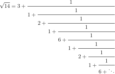
Let’s look at the continued fraction representation for √14.
If we were to take more terms, the sequence of denominators would repeat:
1, 2, 1, 6, 1, 2, 1, 6, 1, 2, 1, 6, …
We could confirm this with Mathematica:
In: ContinuedFraction[Sqrt[14], 13] Out: {3, 1, 2, 1, 6, 1, 2, 1, 6, 1, 2, 1, 6}
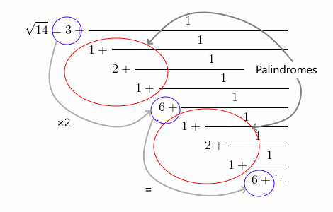
For any integer d that is not a perfect square, the continued fraction for √d has a pattern that we see above.
In the example above, the periodic part is {1, 2, 1, 6}. The palindrome is {1, 2, 1} and 6 is twice the initial coefficient 3.
Another way to state the third point above is to say that the leading coefficient is the integer part of the square root of d, i.e. ⌊√d⌋, and the last coefficient in each period is 2⌊√d⌋.
Sometimes the palindrome is empty:
In: ContinuedFraction[Sqrt[5], 10] Out: {2, 4, 4, 4, 4, 4, 4, 4, 4, 4}
In the continued fraction for √5 the palindrome part is empty and we repeat 4, twice the initial coefficient.
For √3, the palindrome is simply {1} and the final number is 2.
In: ContinuedFraction[Sqrt[3], 13] Out: {1, 1, 2, 1, 2, 1, 2, 1, 2, 1, 2, 1, 2}
One last example:
In: ContinuedFraction[Sqrt[71], 17] Out: {8, 2, 2, 1, 7, 1, 2, 2, 16, 2, 2, 1, 7, 1, 2, 2, 16}
Trott’s constant is the unique number whose digits equal its continued fraction coefficients.
Uniqueness assumes the number is expanded into a simple continued fraction, i.e. one with all numerators equal to 1.
See OEIS sequence A039662.
Every rational number can be expanded into a continued fraction with positive integer coefficients. And the process can be reversed: given a sequence of positive integers, you can make them the coefficients in a continued fraction and reduce it to a simple fraction.
In 1954, Arthur Porges published a one-page article pointing out that continued fractions could be used to create a cipher. To encrypt your cleartext, convert it to a list of integers, use them as continued fraction coefficients, and report the resulting fraction. To decrypt, expand the fraction into a continued fraction and convert the coefficients back to text.
We can implement this in Mathematica as follows:
encode[text_] := FromContinuedFraction[ ToCharacterCode[ text ]] decode[frac_] := FromCharacterCode[ ContinuedFraction[ frac ]]
So, for example, suppose we want to encrypt “adobe.” If we convert each letter to its ASCII code we get {97, 100, 111, 98, 101}. When we make these numbers coefficients in a continued fraction we get
which reduces to 10661292093 / 109898899.
This isn’t a secure encryption scheme by any means, but it’s a cute one. It’s more of an encoding scheme, a (non-secret) way to convert a string of numbers into a pair of numbers.
[1] Arthur Porges. A Continued Fraction Cipher. The American Mathematical Monthly, Vol. 59, No. 4 (Apr., 1952), p. 236
Calendars are based on three frequencies: the rotation of the Earth on its axis, the rotation of the moon around the Earth, and the rotation of the Earth around the sun. Calendars are complicated because none of these periods is a simple multiple of any other. The ratios are certainly not integers, but they’re not even fractions with a small denominator.
As I wrote about the other day in the context of rational approximations for π, the most economical rational approximations of an irrational number come from convergents of continued fractions. The book Calendrical Calculations applies continued fractions to various kinds of calendars.
The continued fraction for the number of days in a year is as follows.
This means that the best approximations for the length of a year are 365 days plus a fraction of 1/4, or 7/29, or 8/33, or 23/95, etc.
You could have one leap day every four years. More accurate would be 7 leap days every 29 years, etc. The Gregorian calendar has 97 leap days every 400 years.
If we express the ratio of the length of the year to the length of the month, we get
By taking various convergents we get 37/3, 99/8, 136/11, etc. So if you want to design successively more accurate lunisolar calendars, you’d have 37 lunar months every 3 years, 99 lunar months every 8 years, etc.
It’s easy to create rational approximations for π. Every time you write down π to a few decimal places, that’s a rational approximation. For example, 3.14 = 314/100. But that’s not the best approximation.
Think of the denominator of your fraction as something you have to buy. If you have enough budget to buy a three-digit denominator, then you’re better off buying 355/113 rather than 314/100 because the former is more accurate. The approximation 355/113 is accurate to 6 decimal places, whereas 314/100 is only accurate to 2 decimal places.
There’s a way to find the most economical rational approximations to π, or any other irrational number, using continued fractions. If you’re interested in details, see the links below.
Here are the 10 best rational approximations to π, found via continued fractions.
|----------------+----------| | Fraction | Decimals | |----------------+----------| | 3 | 0.8 | | 22/7 | 2.9 | | 333/106 | 4.1 | | 355/113 | 6.6 | | 103993/33102 | 9.2 | | 104348/33215 | 9.5 | | 208341/66317 | 9.9 | | 312689/99532 | 10.5 | | 833719/265381 | 11.1 | | 1146408/364913 | 11.8 | |----------------+----------|
If you only want to know the number of correct decimal places, ignore the fractional parts of the numbers in the Decimals column above. For example, 22/7 gives two correct decimal places. But it almost gives three. (Technically, the Decimals column gives the −log10 of the absolute error.)
In case you’re curious, here’s a plot of the absolute errors on a log scale.
The hazard function of a probability distribution is the instantaneous probability density of an event given that it hasn’t happened yet. This works out to be the ratio of the PDF (probability density function) to the CCDF (complementary cumulative density function).
For the standard normal distribution, the hazard function is
and has a surprisingly simple continued fraction representation:
Aside from being an elegant curiosity, this gives an efficient way to compute the hazard function for large x. (It’s valid for any positive x, but most efficient for large x.)
Source: A&S equation 26.2.14
The other day I ran across the following continued fraction for π.
Source: L. J. Lange, An Elegant Continued Fraction for π, The American Mathematical Monthly, Vol. 106, No. 5 (May, 1999), pp. 456-458.
While the continued fraction itself is interesting, I thought I’d use this an example of how to typeset and compute continued fractions.
I imagine there are LaTeX packages that make typesetting continued fractions easier, but the following brute force code worked fine for me:
\pi = 3 + \cfrac{1^2}{6+\cfrac{3^2}{6+\cfrac{5^2}{6+\cfrac{7^2}{6+\cdots}}}}
This relies on the amsmath
package for the \cfrac
command.
Continued fractions of the form
can be computed via the following recurrence. Define A−1 = 1, A0 = a0, B−1 = 0, and B0 = 1. Then for k ≥ 1 define Ak+1 and Bk+1 by
Then the nth convergent the continued fraction is Cn = An / Bn.
The following Python code creates the a and b coefficients for the continued fraction for π above then uses a loop that could be used to evaluate any continued fraction.
N = 20 a = [3] + ([6]*N) b = [(2*k+1)**2 for k in range(0,N)] A = [0]*(N+1) B = [0]*(N+1) A[-1] = 1 A[ 0] = a[0] B[-1] = 0 B[ 0] = 1 for n in range(1, N+1): A[n] = a[n]*A[n-1] + b[n-1]*A[n-2] B[n] = a[n]*B[n-1] + b[n-1]*B[n-2] print( n, A[n], B[n], A[n]/B[n] )
Python uses −1 as a shortcut to the last index of a list. I tack A−1 and B−1 on to the end of the A and B arrays to make the Python code match the math notation. This is either clever or a dirty hack, depending on your perspective.
You may notice that these approximations for π are not particularly good. It’s a trade-off for having a simple pattern to the coefficients. The continued fraction for π that has all b‘s equal to 1 has a complicated set of a‘s with no discernible pattern: 3, 7, 15, 1, 292, 1, 1, etc. However, that continued fraction produces very good approximations. If you replace the first three lines of the code above with that below, you’ll see that four iterations produces an approximation to π good to 10 decimal places.
N = 4 a = [3, 7, 15, 1, 292] b = [1]*N
Take a real number x and expand it as a continued fraction. Compute the geometric mean of the first n coefficients.
Aleksandr Khinchin proved that for almost all real numbers x, as n → ∞ the geometric means converge. Not only that, they converge to the same constant, known as Khinchin’s constant, 2.685452001…. (“Almost all” here mean in the sense of measure theory: the set of real numbers that are exceptions to Khinchin’s theorem has measure zero.)
To get an idea how fast this convergence is, let’s start by looking at the continued fraction expansion of π. In Sage, we can type
continued_fraction(RealField(100)(pi))
to get the continued fraction coefficient
[3, 7, 15, 1, 292, 1, 1, 1, 2, 1, 3, 1, 14, 2, 1, 1, 2, 2, 2, 2, 1, 84, 2, 1, 1, 15, 3]
for π to 100 decimal places. The geometric mean of these coefficients is 2.84777288486, which only matches Khinchin’s constant to 1 significant figure.
Let’s try choosing random numbers and working with more decimal places.
There may be a more direct way to find geometric means in Sage, but here’s a function I wrote. It leaves off any leading zeros that would cause the geometric mean to be zero.
from numpy import exp, mean, log def geometric_mean(x): return exp( mean([log(k) for k in x if k > 0]) )
Now let’s find 10 random numbers to 1,000 decimal places.
for _ in range(10): r = RealField(1000).random_element(0,1) print(geometric_mean(continued_fraction(r)))
This produced
2.66169890535 2.62280675227 2.61146463641 2.58515620064 2.58396664032 2.78152297661 2.55950338205 2.86878898900 2.70852612496 2.52689450535
Three of these agree with Khinchin’s constant to two significant figures but the rest agree only to one. Apparently the convergence is very slow.
If we go back to π, this time looking out 10,000 decimal places, we get a little closer:
print(geometric_mean(continued_fraction(RealField(10000)(pi))))
produces 2.67104567579, which differs from Khinchin’s constant by about 0.5%.