Bitcoin mining difficulty

Posted on 22 February 2026 by John

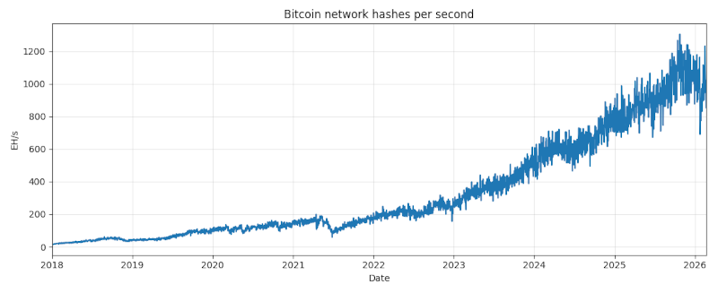
The previous post looked at the Bitcoin network hash rate, currently around one zettahash per second, i.e. 10²¹ hashes per second. The difficulty of mining a Bitcoin block adjusts over time to keep the rate of block production relatively constant, around one block every 10 minutes. The plot below shows this in action.

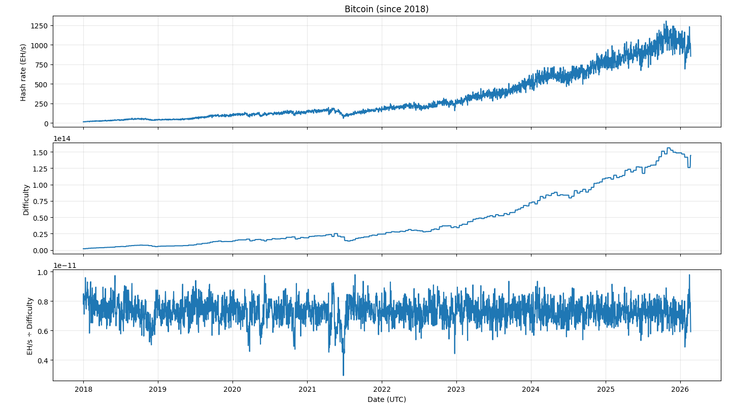
Bitcoin hash rate, difficulty, and ratio of the two

Notice the difficulty graph is more quantized than the hash rate graph. This is because the difficulty changes every 2,016 blocks, or about every two weeks. The number 2016 was chosen to be the number of blocks that would be produced in two weeks if every block took exactly 10 minutes to create.

The ratio of the hash rate to difficulty is basically constant with noise. The noticeable dip in mid 2021 was due to China cracking down on Bitcoin mining. This caused the hash rate to drop suddenly, and it took a while for the difficulty level to be adjusted accordingly.

Mining difficulty

At the current difficulty level, how many hashes would it take to mine a Bitcoin block if there were no competition? How does this compare to the number of hashes the network computes during this time?

To answer these questions, we have to back up a bit. The current mining difficulty is around 10¹⁴, but what does that mean?

The original Bitcoin mining task was to produce a hash [1] with 32 leading zeros. On average, this would take 2³² attempts. Mining difficulty is defined so that the original mining difficult was 1 and current mining difficulty is proportional to the expected number of hashes needed. So a difficulty of around 10¹⁴ means that the expected number of hashes is around

10¹⁴ × 2³² = 4.3 × 10²³.

At one zetahash per second, the number of hashes computed by the entire network over a 10 minute interval would be

10²¹ × 60 × 10 = 6 × 10²³.

So the number of hashes computed by the entire network is only about 40% greater than what would be necessary to mine a block without competition.

[1] The hash function used in Bitcoin’s proof of work is double SHA256, i.e. the Bitcoin hash of x is SHA256( SHA256( x ) ). So a single Bitcoin hash consists of two applications of the SHA256 hash function.

Exahash, Zettahash, Yottahash

Posted on 22 February 2026 by John

When I first heard of cryptographic hash functions, they were called “one-way functions” and seemed like a mild curiosity. I had no idea that one day the world would compute a mind-boggling number of hashes every second.

Because Bitcoin mining requires computing hash functions to solve proof-of-work problems, the world currently computes around 1,000,000,000,000,000,000,000 hashes, one zettahash, per second. Other cryptocurrencies uses hash functions for proof-of-work as well, but they contribute a negligible amount of hashes per second compared to Bitcoin.

The hashrate varies over time because the difficulty of Bitcoin mining is continually adjusted to keep new blocks being produced at about one every ten minutes. As hardware has gotten faster, the difficulty level of mining has gotten higher. When the price of Bitcoin drops and mining becomes less profitable, the difficulty adjusts downward. There are other factors too, and hashrate is variable.

Bitcoin network hashes per second over time

The prefix giga- (10⁹) wasn’t widely known until computer memory and storage entered the gigabyte range. Then the prefix tera- (10¹²) became familiar when disk drives entered terabyte territory. The prefixes for larger units such as peta- (10¹⁵) and exa- (10¹⁸) are still not widely known. The prefixes zetta- (10²¹) and yotta- (10²⁴) were adopted in 1991 and ronna- (10²⁷) and quetta (10³⁰) were adopted in 2022.

When the Bitcoin hashrate is relatively low, it’s in the range of hundreds of exahashes per second. At the time of writing the hashrate is 1.136 ZH/s, 1.136 × 10²¹ hashes per second. This puts the hashrate per day in the tens of yottahashes and the number of hashes per year in tens of ronnahashes.

Bridging secrets is hard

Posted on 30 January 2026 by John

Cryptocurrency and privacy don’t fit together as easily as you might expect. Blockchains give you the illusion of privacy via pseudonymization: you don’t put your name on a blockchain, but you do put information on a blockchain that can be used to determine your name. Blockchain analysis can often reveal information that no one intended to share.

This is true even for privacy coins like Monero and Zcash. These coins put less information directly on chain in the clear, but they still have to be used with skill to maintain privacy. And because they can offer more privacy, they are harder to use. For example, an exchange might let you swap between a thousand different currencies, but privacy coins are conspicuously missing from the list of options. Or maybe you can move money into Zcash, but not with privacy, i.e. not into the shielded pool.

The Privacy trends for 2026 report from a16z summarizes the current situation very well.

Thanks to bridging protocols, it’s trivial to move from one chain to another as long as everything is public. But, as soon as you make things private, that is no longer true: Bridging tokens is easy, bridging secrets is hard. There is always a risk when moving in or out of a private zone that people who are watching the chain, mempool, or network traffic could figure out who you are. Crossing the boundary between a private chain and a public one—or even between two private chains—leaks all kinds of metadata like transaction timing and size correlations that makes it easier to track someone.

As is often the case, the weak link is the metadata, not the data per se.

Prime gaps and Gapcoin

Posted on 18 January 2026 by John

The previous post looked at tightly clustered primes. This post looks at the opposite, large gaps between primes.

Riecoin is a cryptocurrency that uses finding prime clusters as its proof of work task. Gapcoin uses finding prime gaps as its proof of work task.

There’s some nuance to defining prime gaps. It’s trivial to produce a gap of any size. For example, [n! + 2, n! + n] is an interval of length n − 1 that contains no primes. It is more interesting to find gaps that are large relative to the size of the endpoints. The merit of a gap is the ratio of the gap length to the log of the initial number in the interval.

To be specific, suppose p and q are consecutive primes. The length of the gap between them is defined to be q − p and the merit of that gap is (q − p) / log p. For large p, the average gap between primes near p is log p and so the merit function measures how large the gap is relative to what you would expect for the size of p.

The following code will compute the merit function.

>>> from sympy import nextprime, log, N
>>> merit = lambda p: (nextprime(p) - p)/log(p)

Gapcoin adjusts its mining difficulty by adjusting the minimum merit value the miner must search for. Gapcoin miners must find a prime p of the form

p = h × 2^a + b

where h is the SHA256 hash of the previous block in the blockchain and b < 2^a.

The prime gap with the largest known merit is [p, p + 8350] where

p = 293703234068022590158723766104419463425709075574811762098588798217895728858676728143227

The code

>>> N(merit(p))

shows that the merit is 41.94.

This record was found by the Gapcoin network. I don’t know the backstory, but I presume the mining task wasn’t to find a world record gap. Instead, the miner got lucky and found a much larger gap than necessary.

Prime clusters and Riecoin

Posted on 18 January 2026 by John

Prime clusters are sets of primes that appear as close together as is generally possible.

There is one pair of consecutive prime numbers, 2 and 3, but there cannot be any more: in any larger pair of consecutive numbers, one of the pair will be even. But there are a lot of twin primes, perhaps infinitely many, and so a prime cluster of size two is a pair of primes whose difference is 2.

How close together can a set of three primes be? The set {2, 3, 5} has diameter 3, i.e. the difference between the largest and smallest element is 3. And the set {3, 5, 7} has diameter 4. But in general the diameter of a set of three primes must be at least 6. If the smallest element is bigger than 3, then all the elements are odd, but they cannot be consecutive odd numbers or else one of them would be divisible by 3. But there are many prime clusters of diameter 6. For example, {13, 17, 19} and {37, 41, 43}.

Formal definition and motivation

There is some fuzziness in the discussion above regarding what is generally possible. This section will make our definitions more rigorous.

In general a pair of primes cannot be consecutive numbers because one of the pair must be even. Stated more abstractly, every pair of integers larger than {2, 3} will contain a complete residue class mod 2, i.e. one of the numbers will be congruent to 0 mod 2 and one of the numbers will be congruent to 1 mod 2.

Now let’s look at sets of three primes. The example {2, 3, 5} is exceptional because it contains a complete residue class mod 2, i.e. it contains even and odd numbers. The example {3, 5, 7} is exceptional because it contains a complete residue class mod 3.

We say that a set of k primes is a cluster if it does not contain a full residue class modulo any prime. We could say it does not contain a full residue class modulo any prime q ≤ k because trivially no set of k elements can have set of more than k elements. For example, the cluster {13, 17, 19} does not contain a full set of residues mod 2 or 3, but it also does not have a full set of residues mod 5, 7, 11, ….

We say a cluster is maximally dense if it has the minimum diameter for a cluster of its number of primes.

Informally, we will call a maximally dense cluster simply a cluster. A maximally dense prime cluster is also sometimes called a prime constellation.

Riecoin cryptocurrency

I’ve written several posts about the Primecoin cryptocurrency whose proof of work task is finding prime chains. The Riecoin cryptocurrency requires miners to find prime clusters.

Primecoin is far from a major cryptocurrency, with a market cap of around $2.3M. Riecoin is about four times smaller than Primecoin. There is another number-theoretic cryptocurrency, Gapcoin, whose market cap is about 10x smaller than that of Riecoin. Safe to say these three projects are of more interest to mathematicians than investment firms. All three of these prime-based cryptocurrencies were launched between 2013 and 2014.

A proof of work task should satisfy three criteria:

Solutions should be difficult to find but easy to confirm.
The time to find a solution should be roughly predictable.
The difficulty should be adjustable.

Finding prime clusters requires a brute force search, but it’s easy to test whether a cluster has been found, and so the first property is satisfied.

The Hardy-Littlewood conjectures give an estimate of the difficulty in finding prime clusters of a given length. The difficulty can be adjusted by adjusting the required length. So the Hardy-Littlewood conjectures assist in satisfying the second and third properties. It does not matter if the conjectures are false somewhere out in asymptopia; they empirically give good estimates for the size of numbers used in mining Riecoin.

More about clusters

The definition of a maximally dense cluster depends on a function s(k) that says what the diameter of a cluster of k primes would need to be. We’ve said s(2) = 2 and s(3) = 6. More values of s are listed on the page for OEIS sequence A008407.

Prime chains

Posted on 10 January 2026 by John

The title of this post has a double meaning. We will look at chains in the sense of number theory and in the sense of cryptocurrency, i.e. Cunningham chains and blockchains, that involve prime numbers.

Cunningham chains

A chain of primes is a sequence of prime numbers in which each is almost double its predecessor. That is, the next number after p is 2p ± 1.

In a Cunningham chain of the first kind, the successor of p is 2p + 1. For example,

41, 83, 167.

In a Cunningham chain of the second kind, the successor of p is 2p − 1. For example,

19, 37, 73.

Two questions come up immediately. First, are there infinitely many Cunningham chains? Second, how long can a Cunningham chain be? What is known and what is conjectured are at opposite ends of the spectrum. It is unknown whether there are infinitely many Cunningham chains of length 2, but it is conjectured that there are infinitely many Cunningham chains of all lengths.

According to this page, the longest known Cunningham chains of the first kind has length 17, and the longest known Cunningham chain of the second kind has length 19. We can verify these results with the following Python code.

from sympy import isprime

def chain_length(start, kind):
    p = start
    c = 0
    while isprime(p):
        c += 1
        p = 2*p + kind
    return c

print(chain_length(2759832934171386593519, 1))
print(chain_length(79910197721667870187016101, -1))

Bi-twin chains

A number n is the basis of a bi-twin chain of length k if n − 1 is the start of a Cunningham chain of the first kind of length k and n + 1 is the start of a Cunningham chain of the second kind of length k.

I say more about bi-twin prime chains in the next post.

Primecoin

Primecoin was one of the first cryptocurrencies, coming out four years after Bitcoin. Primecoin is still going, though its market cap is six orders magnitude smaller than that of Bitcoin.

What’s interesting about Primecoin is that it uses finding prime chains as its proof of work task [1]. To mint a new Primecoin block, you must find a prime chain of the required length whose origin a multiple of the hash of the block header [2].

Primecoin allows any of the three kinds of prime chains mentioned above: Cunningham chains of the first or second kind, or a bi-twin prime chain. Primecoin adjusts its mining difficulty over time by varying the length of Cunningham or bi-twin chain needed to mint a new block.

There are also cryptocurrencies based on finding prime clusters and prime gaps.

[1] Strictly speaking, Primecoin requires finding probable prime chains, as explained here.

[2] The origin of a prime chain is n if the first item in a Cunningham chain of the first kind is n + 1, or if the first item in a Cunningham chain of the first kind or a bi-twin chain is n − 1.

Compressing a set of hash values

Posted on 9 January 2026 by John

Suppose you have a set of k hash values, each n bits long. Can you compress the set into less than kn bits?

It’s not possible to compress a list of hashes into less than kn bits, but you can hash a set into fewer bits.

Suppose you have a set of 2³⁰, roughly a billion, 64-bit hashes. Sort the set and look at the size of gaps between elements. You might expect that consecutive items on the list are roughly 2³⁴ apart, and so you could reconstruct the list by reporting the first item and the gaps between the rest, which are 34-bit numbers, not 64-bit numbers, a savings of 30 bits per hash.

This doesn’t exactly work, but it’s the kernel of a good idea. We don’t know that the distance between hashes can be represented by a 34 bit number. The gap could be more or less than 2³⁴, but we don’t expect it to often be much more than 2³⁴. So we use a variable-length encoding such that when the distance between values is on the order of 2³⁴, or less, we save bits, but we allow for the distance to be any size.

Applications

What we’ve described is the essence of Golomb-Rice coding. Its implementation in the Bitcoin protocol is referred to as Golomb-Coded Sets (GCS), described in BIP 158. Golomb-Rice coding is also used other applications where the values to be compressed are not hashes, such as in lossless auto compression.

Encoding

Let’s go into some detail as to how the distances between sorted values are represented. Suppose you expect the differences to be on the order of M where M is a power of 2. For each difference d, let q and r be the quotient and remainder by M, i.e.

d = qM + r.

Encode q as a unary number, i.e. string of q 1s, and encode r as an ordinary binary number. Then Golomb-Rice coding of d is the concatenation of the representations of q and r. with a 0 in the middle as a separator. Using || to denote string concatenation we have

unary(q) || 0 || binary(r).

In general, unary encoding is extremely inefficient, but we’re betting that q will typically be quite small.

The reason we require M to be a power of 2 is so the representation of r will have a fixed length [1].

Let’s work out an example. Suppose M = 2²⁰ and

d = 2²² + 123456 = 4 × M + 123456.

Then we write q as 1111 and r as 0011110001001000000 and encode d as the string

111100011110001001000000

Decoding

You can concatenate the encodings of consecutive d values and still be able to unambiguously decode the result. Because the r representations have a constant length, you know when an r ends and the next q begins.

For example, suppose we have the following string of bits.

1110010011001011001011111001000000110010001110011101111000101111011

We decode the string from left to right. We count how many ones we see, skip over a 0, then regarding the next 20 bits as a binary number.

111 0 01001100101100101111 1 0 01000000110010001110 0 11101111000101111011

We see three 1s before the first 0 and so we conclude q₁ = 3. We skip over the 0 and read the value of r.

r₁ = 01001100101100101111_two = 314159.

Next we see a single 1 before the next 0, so q₂ = 1. We read the next value of r as

r₂ = 01000000110010001110_two = 265358.

Next we see a 0, i.e. there are no 1s, and so the final q₃ = 0. And we have

r₃ = 11101111000101111011_two = 979323.

So our reconstructed values of d are

d₁ = q₁ M+ r₁ = 3 × 2²⁰ + 314159 = 3459887

d₂ = q₂ M+ r₂ = 1 × 2²⁰ + 265358 = 1313934

d₃ = q₃ M+ r₃ = 0 × 2²⁰ + 979323 = 979323.

Now these are difference values. We need to know the smallest value m in order to construct the original set of values from the differences. Then the full values are m, m + d₁, m + d₁ + d₂, and m + d₁+ d₂+ d₃,.

[1] This is the Rice part. Robert Rice simplified Samuel Golomb’s encoding scheme in the special case that M is a power of 2.

Obscuring P2P nodes with Dandelion

Posted on 8 December 2025 by John

The weakest link in the privacy of cryptocurrency transactions is often outside the blockchain. There are technologies such as stealth addresses and subaddresses to try to thwart attempts to link transactions to individuals. They do a good job of anonymizing transaction data, but the weak link may be metadata, as is often the case.

Cryptocurrency nodes circulate transaction data using a peer-to-peer network. An entity running multiple nodes can compare when data arrived at each of its nodes and triangulate to infer which node first sent a set of transactions. The Dandelion protocol, and its refinement Dandelion++, aims to mitigate this risk. Dandelion++ is currently used in Monero and a few other coins; other cryptocurrencies have considered or are considering using it.

Dandelion plant

The idea behind the Dandelion protocol is to have a “stalk” period and a “diffusion” period. Imagine data working up the stalk of a dandelion plant before diffusing like seeds in the wind. The usual P2P process is analogous to simply blowing on the seed head [1].

During the stalk period, information travels from one node to one node. Then after some number of hops, the diffusion process begins; the final node in the stalk period diffuses the information to all its peers. An observer with substantial but not complete visibility of the network may be able to determine which node initiated the diffusion, but maybe not the node at the other end of the stem.

A natural question is how this differs from something like Tor. In a nutshell, Tor offers identity protection before you enter a P2P network, and Dandelion offers identity protection inside the P2P network.

For more details, see the original paper on Dandelion [2].

[1] The original paper on Dandelion uses a dandelion seed as the metaphor for the protocol. “The name ‘dandelion spreading’ reflects the spreading pattern’s resemblance to a dandelion seed head and refers to the diagram below. However, other sources refer to the stalk and head of the dandelion plant, not just a single seed. Both mental images work since the plant has a slightly fractal structure with a single seed looking something like the plant.

Illustration from Dandelion protocol paper

[2] Shaileshh Bojja Venkatakrishnan, Giulia Fanti, Pramod Viswanath. Dandelion: Redesigning the Bitcoin Network for Anonymity. Proceedings of the ACM on Measurement and Analysis of Computing Systems, Volume 1, Issue 1 Article No.: 22, Pages 1–34. Available here: https://doi.org/10.1145/3084459.

What is a Pedersen commitment?

Posted on 6 December 2025 by John

I’m taking a break from my series on celestial navigation. The previous posts give the basics, but I haven’t thought of a way to go further that I’m satisfied with. So now for something completely different: Pedersen commitments.

Pedersen commitments are a building block of zero knowledge proofs (ZKP), and they give an opportunity to look at a couple other interesting topics: nothing-up-my-sleeve constructions and homomorphic encryption.

A Pedersen commitment to a value v takes a random number x and two generators of an elliptic curve, G and H, and returns

C = vG + xH.

The significance of C is that it appears to be a random number to the recipient, but the sender who calculated it can later show that it was computed from v and x. C is called a commitment to the value v because the sender cannot later say that C was computed from a different v and a different x.

Mathematical details

The addition in

C = vG + xH

is carried out on an elliptic curve, such as Ed25519 in the case of Monero. Multiplication is defined by repeated addition, though it’s not computed that way [1]. G and H are not just points on the elliptic curve but points in a large, prime-order subgroup of the elliptic curve.

Because the value x is random, the possible values of C are uniformly distributed on the curve, and so someone observing C learns nothing about v. For that reason x is called a blinding factor.

The difficulty of the discrete logarithm problem insures that it is impractical come up with different values v‘ and x‘ such that

v G + x H = v‘ G + x‘ H.

This depends on two assumptions.

The first assumption is that the discrete logarithm problem is hard to solve given current algorithms and hardware. The prevailing opinion is that it is unlikely anyone will come up with an efficient algorithm for solving the discrete logarithm problem on current hardware. However, Shor’s algorithm could solve the discrete logarithm problem efficiently if and when a practical, large-scale quantum computer is created.

The second assumption is that the generator H was chosen at random and not calculated to be a backdoor.

How to make and use a backdoor

Because G and H are members of the same prime-order (i.e. cyclic) group, there exists some integer h such

H = hG

If the generator H was randomly selected, nobody knows h and nobody can calculate it. But if H was calculated by first selecting h and multiplying hG then there is a backdoor.

Now

C = vG + xH = vG + x(hG) = (v + xh)G.

If you know h, you can pick a new v‘ and solve for x‘ such that

v + xh = v‘ + x‘ h.

That would mean that in the context of a cryptocurrency that uses Pedersen commitments, such as Monero or the Liquid Network on top of Bitcoin, you could initially commit to spending v and later claimed that you committed to spending v‘.

Note that solving for x‘ requires modular arithmetic, not solving the discrete logarithm problem.

How to prove no backdoor

The way to prove that the generator H was chosen in good faith is to be transparent about how it was created. In practice this means using some sort of cryptographic hash function. For example, Bulletproofs hashed “bulletproof_g” and “bulletproof_h” to create its values of G and H. Bulletproofs require multiple values of G and H and so consecutive integers were concatenated to the strings before hashing.

Reversing a cryptographic hash like SHA256 is impractical, even assuming you have a quantum computer, and so it is extremely unlikely that there is a backdoor when the generators were created by hashing a natural string.

It’s said that Pedersen commitments do not require a trusted setup. That’s true in spirit, but more precisely they require a transparent setup that is easy to trust.

Homomorphic encryption

The function

C: (v, x) ↦ vG + xH

is a group homomorphism from pairs of integers to the subgroup generated by G and H. This means that

C(v, x) + C(v‘, x‘) = C(v + v‘, x + x‘)

or in other words, you can combine multiple commitments into a single commitment. The sum of a commitment to (v, x) and a commitment to (v‘, x‘) is a commitment to (v + v‘, x + x‘).

[1] In practice the number x is enormous, say on the order of the number of points on the elliptic curve, and so software does not add H to itself x times. Instead it uses a process analogous to fast exponentiation. In fact, if you write the group operation multiplicatively rather than additively, it is exactly fast exponentiation.

Monero subaddresses

Posted on 28 November 2025 by John

Monero has a way of generating new addresses analogous to the way HD wallets generate new addresses for Bitcoin. In both cases, the recipient’s software can generate new addresses to receive payments that others cannot link back to the recipient.

Monero users have two public/private keys pairs: one for viewing and one for spending. Let K^s and k^s be the public and private spending keys, and let K^v and k^v be the public and private viewing keys. Then the user’s ith subaddress is given by

$\begin{align*} K^s_i &= K^s + H(k^v, i) G \\ K^v_i &= k^v K^s_i \end{align*}$

Here G is a generator for the elliptic curve Ed25519 and H is a hash function. The hash function output and k^v are integers; the public keys, denoted by capital Ks with subscripts and superscripts, are points on Ed25519. The corresponding private keys are

$\begin{align*} k^s_i &= k^s + H(k^v, i) \\ k^v_i &= k^v + k^s_i \end{align*}$

As with hierarchical wallets, the user scans the blockchain to see which of his addresses have received funds.

A user may choose to give a different subaddress for each transaction for added security, or to group transactions for accounting purposes.

Note that in addition to subaddresses, Monero uses stealth addresses. An important difference between subaddresses and stealth addresses is that recipients generate subaddresses, and senders generate stealth addresses. Someone could send you money to the same subaddress twice, failing to create a new stealth address. This is not possible if you give the sender a different subaddress each time.

Janus attacks

The possibility of a Janus attack is a fly in the subaddress ointment. If an attacker suspects that two subaddresses belong to the same wallet, they can confirm this suspicion by sending a transaction to one subaddress and making it look like it came from the other. If the recipient confirms receipt of the funds, they inform the attacker that his suspicion was correct. A cautious user might not confirm receipt of funds, but a cryptocurrency exchange would. You can read more about the details of a Janus attack here.

Cryptocurrency

Bitcoin mining difficulty

Mining difficulty

Related posts

Exahash, Zettahash, Yottahash

Related posts

Bridging secrets is hard

Prime gaps and Gapcoin

Related posts

Prime clusters and Riecoin

Formal definition and motivation

Riecoin cryptocurrency

More about clusters

Related posts

Prime chains

Cunningham chains

Bi-twin chains

Primecoin

Related posts

Compressing a set of hash values

Applications

Encoding

Decoding

Related posts

Obscuring P2P nodes with Dandelion

Related posts

What is a Pedersen commitment?

Mathematical details

How to make and use a backdoor

How to prove no backdoor

Homomorphic encryption

Related posts

Monero subaddresses

Janus attacks

Related posts