I’ve written a couple times about Fibonacci numbers and certificates. Here the certificate is auxiliary data that makes it faster to confirm that the original calculation was correct.
This post puts some timing numbers to this.
I calculated the 10 millionth Fibonacci number using code from this post.
n = 10_000_000
F = fib_mpmath(n)
This took 150.3 seconds.
As I’ve discussed before, a number f is a Fibonacci number if and only if 5f² ± 4 is a square r². And for the nth Fibonacci number, we can take ± to be positive if n is even and negative if n is odd.
I computed the certificate r with
r = isqrt(5*F**2 + 4 - 8*(n%2))
and this took 65.2 seconds.
Verifying that F is correct with
n = abs(5*F**2 - r**2)
assert(n == 4)
took 3.3 seconds.
About certificates
So in total it took 68.5 seconds to verify that F was correct. But if someone had pre-computed r and handed me F and r I could use r to verify the correctness of F in 3.3 seconds, about 2% of the time it took to compute F.
Sometimes you can get a certificate of correctness for free because it is a byproduct of the problem you’re solving. Other times computing the certificate takes a substantial amount of work. Here computing F and r took about 40% more work than just computing F.
What’s not typical about this example is that the solution provider carries out exactly the same process to create the certificate that someone receiving the solution without a certificate would do. Typically, even if the certificate isn’t free, it does come at a “discount,” i.e. the problem solver could compute the certificate more efficiently than someone given only the solution.
Proving you have the right Fibonacci number
Now suppose I have you the number F above and claim that it is the 10,000,000th Fibonacci number. You carry out the calculations above and say “OK, you’ve convinced me that F is a Fibonacci number, but how do I know it’s the 10,000,000th Fibonacci number?
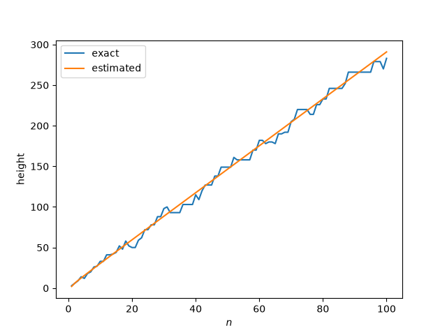
The 10,000,000th Fibonacci number has 2,089,877 digits. That’s almost enough information to verify that a Fibonacci number is indeed the 10,000,000th Fibonacci number. The log base 10 of the nth Fibonacci number is very nearly
n log10 φ − 0.5 log10 5
based on Binet’s formula. From this we can determine that the nth Fibonacci number has 2,089,877 digits if n = 10,000,000 + k where k equals 0, 1, 2, or 3.
Because
log10 F10,000,000 = 2089876.053014785
and
100.053014785 = 1.129834377783962
we know that the first few digits of F10,000,000 are 11298…. If I give you a 2,089,877 digits that you can prove to be a Fibonacci number, and its first digit is 1, then you know it’s the 10,000,000th Fibonacci number.
You could also verify the number by looking at the last digit. As I wrote about here, the last digits of Fibonacci number have a period of 60. That means the last digit of the 10,000,000th Fibonacci number is the same as the last digit of the 40th Fibonacci number, which is 5. That is enough to rule out the other three possible Fibonacci numbers with 2,089,877 digits.