Additive and multiplicative persistence

Casting out nines is a well-known way of finding the remainder when a number is divided by 9. You add all the digits of a number n. And if that number is bigger than 9, add all the digits of that number. You keep this up until you get a number less than 9.

This is an example of persistence. The persistence of a number, relative to some operation, is the number of times you have to apply that operation before you reach a fixed point, a point where applying the operation further makes no change.

The additive persistence of a number is the number of times you have to take the digit sum before getting a fixed point (i.e. a number less than 9). For example, the additive persistence of 8675309 is 3 because the digits in 8675309 sum to 38, the digits in 38 sum to 11, and the digits in 11 sum to 2.

The additive persistence of a number in base b is bounded above by its iterated logarithm in base b.

The smallest number with additive persistence n is sequence A006050 in OEIS.

Multiplicative persistence is analogous, except you multiply digits together. Curiously, it seems that multiplicative persistence is bounded. This is true for numbers with less than 30,000 digits, and it is conjectured to be true for all integers.

The smallest number with multiplicative persistence n is sequence A003001 in OEIS.

Here’s Python code to compute multiplicative persistence.

def digit_prod(n):
    s = str(n)
    prod = 1
    for d in s:
        prod *= int(d)
    return prod

def persistence(n):
    c = 0
    while n > 9:
        n = digit_prod(n)
        print(n)
        c += 1
    return c   

You could use this to verify that 277777788888899 has persistence 11. It is conjectured that no number has larger persistence larger than 11.

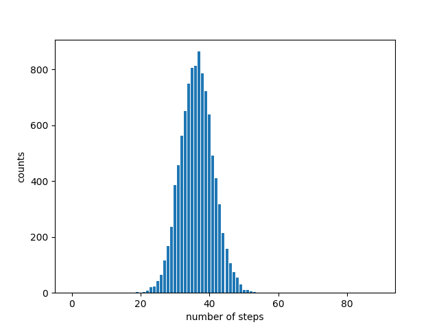
The persistence of a large number is very likely 1. If you pick a number with 1000 digits at random, for example, it’s very likely that at least of these digits will be 0. So it would seem that the probability of a large number having persistence larger than 11 would be incredibly small, but I would not have expected it to be zero.

Here are plots to visualize the fixed points of the numbers less than N for increasing values of N.


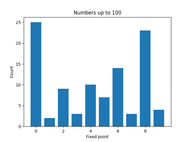
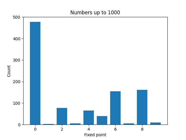
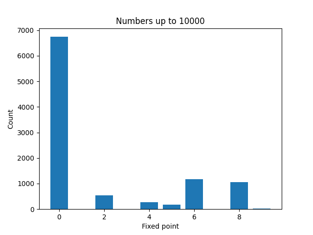
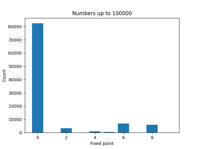
It’s not surprising that zeros become more common as N increases. And a moments thought will explain why even numbers are more common than odd numbers. But it’s a little surprising that 4 is much less common than 2, 6, or 8.

Incidentally, we have worked in base 10 so far. In base 2, the maximum persistence is 1: when you multiply a bunch of 0s and 1s together, you either get 0 or 1. It is conjectured that the maximum persistence in base 3 is 3.

False witnesses

Pinocchio talking to a judge

Fermat’s primality test

Fermat’s little theorem says that if p is a prime and a is not a multiple of p, then

ap−1 = 1 (mod p).

The contrapositive of Fermat’s little theorem says if

ap−1 ≠ 1 (mod p)

then either p is not prime or a is a multiple of p. The contrapositive is used to test whether a number is prime. Pick a number a less than p (and so a is clearly not a multiple of p) and compute ap−1 mod p.  If the result is not congruent to 1 mod p, then p is not a prime.

So Fermat’s little theorem gives us a way to prove that a number is composite: if ap−1 mod p equals anything other than 1, p is definitely composite. But if ap−1 mod p does equal 1, the test is inconclusive. Such a result suggests that p is prime, but it might not be.

Examples

For example, suppose we want to test whether 57 is prime. If we apply Fermat’s primality test with a = 2 we find that 57 is not prime, as the following bit of Python shows.

    >>> pow(2, 56, 57)
    4

Now let’s test whether 91 is prime using a = 64. Then Fermat’s test is inconclusive.

    >>> pow(64, 90, 91)
    1

In fact 91 is not prime because it factors into 7 × 13.

If we had used a = 2 as our base we would have had proof that 91 is composite. In practice, Fermat’s test is applied with multiple values of a (if necessary).

Witnesses

If ap−1 = 1 (mod p), then a is a witness to the primality of p. It’s not proof, but it’s evidence. It’s still possible p is not prime, in which case a is a false witness to the primality of p, or p is a pseudoprime to the base a. In the examples above, 64 is a false witness to the primality of 91.

Until I stumbled on a paper [1] recently, I didn’t realize that on average composite numbers have a lot of false witnesses. For large N, the average number of false witnesses for composite numbers less than N is greater than N15/23. Although N15/23 is big, it’s small relative to N when N is huge. And in applications, N is huge, e.g. N = 22048 for RSA encryption.

However, your chances of picking one of these false witnesses, if you were to choose a base a at random, is small, and so probabilistic primality testing based on Fermat’s little theorem is practical, and in fact common.

Note that the result quoted above is a lower bound on the average number of false witnesses. You really want an upper bound if you want to say that you’re unlikely to run into a false witness by accident. The authors in [1] do give upper bounds, but they’re much more complicated expressions than the lower bound.

Related posts

[1] Paul Erdős and Carl Pomerance. On the Number of False Witnesses for a Composite Number. Mathematics of Computation. Volume 46, Number 173 (January 1986), pp. 259–279.

The bad version of a good test

Ever since 1952, the largest known primes have all had the form 2n − 1, with one exception in 1989. The reason the largest known primes have this form is that it is easier to test whether these numbers are prime than other numbers.

A number of the form 2n − 1 is called a Mersenne number, denoted Mn. A Mersenne prime is a Mersenne number that is also prime. There is a theorem that says that if Mn is prime then n must be prime.

Lehmer’s theorem

Derrick Henry Lehmer proved in 1930 that Mp is prime if p is an odd prime and Mp divides sp−2 where the s terms are defined recursively as follows. Define s0 = 4 and sn = sn−1² − 2 for n > 0. This is the Lucas-Lehmer primality test for Mersenne numbers, the test alluded to above.

Let’s try this out on M7 = 27 − 1 = 127. We need to test whether 127 divides s5. The first six values of sn are

4, 14, 194, 37634, 1416317954, 2005956546822746114

and indeed 127 does divide 2005956546822746114. As you may have noticed, s5 is a big number, and s6 will be a lot bigger. It doesn’t look like Lehmer’s theorem is going to be very useful.

The missing piece

Here’s the idea that makes the Lucas-Lehmer [1] test practical. We don’t need to know  sp−2 per se; we only need to know whether it is divisible by Mp. So we can carry out all our calculations mod Mp. In our example, we only need to calculate the values of sn mod 127:

4, 14, 67, 42, 111, 0

Much better.

Lucas-Lehmer test takes the remainder by Mp at every step along the way when computing the recursion for the s terms. The naive version does not, but computes the s terms directly.

To make the two versions of the test explicit, here are Python implementations.

Naive code

def lucas_lehmer_naive(p):
    M = 2**p - 1
    s = 4
    for _ in range(p-2):
        s = (s*s - 2) 
    return s % M  == 0

Good code

def lucas_lehmer(p):
    M = 2**p - 1
    s = 4
    for _ in range(p-2):
        s = (s*s - 2) % M
    return s == 0

The bad version

How bad is the naive version of the Lucas-Lehmer test?

The OEIS sequence A003010 consists of the sn. OEIS gives the following formula:

s_n = \left\lceil (2 + \sqrt{3})^{2^n}\right\rceil

This shows that the sn grow extremely rapidly, which suggests the naive algorithm will hit a wall fairly quickly

When I used the two versions of the test above to verify that the first few Mersenne primes Mp really are prime, the naive version gets stuck after p = 19. The better version immediately works through p = 9689 before slowing down noticeably.

Historical example

Let’s look at M521. This was the first Mersenne number verified by a computer to be prime. This was done on the vacuum tube-based SWAC computer in 1952 using the smart version of the Lucas-Lehmer test.

Carrying out the Lucas-Lehmer test to show that this number is prime requires doing modular arithmetic with 521-bit numbers, which was well within the 9472 bits of memory in the vacuum tube-based SWAC computer that proved M521 was prime.

But it would not be possible now, or ever, to verify that M521 is prime using the naive version of the Lucas-Lehmer test because we could not store, much less compute, s519.

Since

\log_{2} s_{519} = 2^{519} \log_{2} (2 + \sqrt{3}) \approx 2^{520}

we’d need around 2520 bits to store s519. The number of bits we’d need is itself a 157-digit number. We’d need more bits than there are particles in the universe, which has been estimated to be on the order of 1080.

The largest Mersenne prime that the SWAC could verify using the naive Lucas-Lehmer test would have been M13 = 8191, which was found to be prime in the Middle Ages.

Related posts

[1] Édouard Lucas conjectured in 1878 the theorem that Lehmer proved in 1930.

Distribution of run times for Euclidean algorithm

The worst case run time for the Euclidean algorithm occurs when you give the algorithm a pair of consecutive Fibonacci numbers. The algorithm takes n steps to compute the greatest common divisor of Fn+1 and Fn+2.

The nth Fibonacci number is the nearest integer to φn/√5 where φ = (1 + √5)/2 is the golden ratio. You can take logs and solve for the largest n such that Fn is less than x, subtract 2, and have an upper bound on the number of steps necessary to find the gcd of two numbers less than x.

But what about the average run time, or the distribution of run times?

For large x, the distribution of number of steps needed to calculate the gcd of two numbers 0 < abx using the Euclidean algorithm is approximately normal with mean

12 log(2) log(x) / π².

See, for example, [1].

Let’s illustrate this with a simulation. Here’s Python code to return the number of steps used in computing gcd(ab).

    def euclid(a, b):
        steps = 0
        while a != 0:
            a, b = b%a, a
            steps += 1
        return steps # gcd = b

I generated 10,000 pairs of random integers less than 263 (because the maximum signed 64 bit integer is 263 − 1) and plotted a histogram of the run times.

I got a nice bell curve with mean 36.3736. The theoretical mean is 0.8428 log(263) = 36.8021.

[1] Doug Hensley. The Number of Steps in the Euclidean Algorithm. Journal of Number Theory 49. 142–182 (1994).

Equipentatonic scale

I ran across a video that played around with the equipentatonic scale [1]. Instead of dividing the octave into 12 equal parts, as is most common in Western music, you divide the octave into 5 equal parts. Each note in the equipentatonic scale has a frequency 21/5 times its predecessor.

The equipentatonic scale is used in several non-Western music systems. For example, the Javanese slendro tuning system is equipentatonic, as is Babanda music from Uganda.

In the key of C, the nearest approximants of the notes in the equipentatonic scale are C, D, F, G, A#. Approximate equipentatonic scale

In the image above [2], the D is denoted as half sharp, 50 cents higher than D. (A cent is 1/100 of a half step.) The actual pitch is a D plus 40 cents, so the half sharp is closer, but still not exactly right.

The F should be 20 cents lower, the G should be 20 cents higher, and the A# should be 10 cents higher.

Notation

The conventional chromatic scale is denoted 12-TET, an abbreviation for 12 tone equal temperament. In general n-TET denotes the scale that results from dividing the octave into n parts. The previous discussion was looking at how 5-TET aligns with 12-TET.

A step in 5-TET corresponds to 2.4 steps in 12-TET. This is approximately 5 steps in 24-TET, the scale we’d get by adding quarter tones between all the notes in the chromatic scale.

Math

When we talk of dividing the octave evenly into n parts, we mean evenly on a logarithmic scale because we perceive music on a log scale.

The notation will be a little cleaner if we start counting from 0. Then the kth note the n-TET scale is proportional to 2k/n.

The proportionality constant is the starting pitch. So if we start on middle C, the frequencies are 262 × 2k/n Hz. The nth frequency is twice the starting frequency, i.e. an octave higher.

We can measure how well an m-TET scale can be approximated by notes from an n-TET scale with the following function:

d(m, n) = \max_j \min_k \left|\frac{j}{m} - \frac{k}{n} \right|

Note that this function is asymmetric: d(mn) does not necessarily equal d(nm). For example, d(12, 24) = 0 because a quarter tone scale contains exact matches for every note in a semitone scale. But d(24, 12) = 1/24 because the quarter tone scale contains notes in between the notes of the semitone scale.

The equipentatonic scale lines up better with the standard chromatic scale than would a 7-note scale or an 11-note scale. That is, d(5, 12) is smaller than d(7, 12) or d(11, 12). Something similar holds if we replace 12 with 24: d(5, 24) is smaller than d(m, 24) for any m > 1 that is relatively prime to 24.

Related posts

[1] The video first presents 10-TET and then defines 5-TET as taking every other note from this scale.

[2] The image was created with the following Lilypond code.

\score {
  \new Staff {
    \relative c' {
      c1 dih f g aih c \bar "|."
    }
  }
  \layout {
    \context {
      \Staff
      \remove "Bar_engraver"
      \remove "Time_signature_engraver"
    }
  }
}

When Benford’s law is exact

Eight years ago I wrote a blog post on the Leading digits of powers of 2. In that post I said that Benford’s law gives remarkably good predictions for the distribution of leading digits of 2n. In this post I’ll make that statement stronger.

A sequence obeys Benford’s law, in base 10, if the proportion of the first N elements of the sequence that begin with the digit d is asymptotically

N log10(1 + 1/d).

Benford’s law applies to powers of 2, but also to factorials, for example. In general it applies only in the limit as N goes to infinity. For a large but finite value of N it gives a good approximation, but there’s no guarantee on how good the approximation is.  Except sometimes there is.

You could use Benford’s law to estimate how many times n! begins with a 1, but it can tell you exactly how many times 2n begins with a 1. The exact number is the estimate given by Benford’s law with d = 1, rounded down to the nearest integers, i.e. the floor of the expression above.

N log10(2)⌋

See [1] for a proof. The following Python code demonstrates this.

    import decimal
    from math import log10, floor

    def exact(N):
        c = 0
        a = decimal.Decimal(1)
        for i in range(1, N+1):
            a = a*2
            if int(str(a)[0]) == 1:
                c += 1
        return c

    def estimated(N):
        return N*log10(2)

    for i in range(1, 10000):
        assert(exact(i) == int(floor(estimated(i))))

The code uses the decimal class for efficiency. See Andrew Dalke’s comment on the original post. [2]

Benford’s law predicts exactly how often the sequence 2n begins with a 1. It also predicts exactly how often it begins with 4, but it is not exact for other digits.

Related posts

[1] Zhaodong Cai, Matthew Faust, A. J. Hildebrand, Junxian Li, Yuan Zhang. The Surprising Accuracy of Benford’s Law in Mathematics. The American Mathematical Monthly, Vol. 127, No. 3 (MARCH 2020), pp. 217–237

[2] The function exact is efficient for individual values of N, but there is a lot of redundant calculation when you use it to test a range of N‘s as we do in the loop with the assert statement. It wouldn’t be hard to rewrite the code to have it more efficiently check a range.

The Buenos Aires constant

The Buenos Aires constant is 2.92005097731613…

What’s so special about this number? Let’s see when we use it to initialize the following Python script.

s = 2.920050977316134

for _ in range(10):
    i = int(s)
    print(i)
    s = i*(1 + s - i)

What does this print?

    2, 3, 5, 7, 11, 13, 17, 19, 23, 29

If we started with the exact Buenos Aires constant and carried out our operations exactly, the procedure above would generate all prime numbers. In actual IEEE 754 arithmetic, it breaks down around Douglas Adams’ favorite number.

The Buenos Aires constant is defined by the infinite sum

\lambda = \frac{2-1}{1} + \frac{3-1}{2} + \frac{5-1}{3\cdot 2} + \frac{7-1}{5\cdot 3 \cdot 2} + \cdots

As you can tell, the primes are baked into the definition of λ, so the series can’t generate new primes.

I used mpmath to calculate λ to 100 decimal places:

2.920050977316134712092562917112019468002727899321426719772682533107733772127766124190178112317583742

This required carrying out the series defining λ for the first 56 primes. When I carried out the iteration above also to 100 decimal places, it failed on the 55th prime. So I got about as many primes out of the computation as I put into it.

Related posts

Reference: Beyond Pi and e: a Collection of Constants. James Grime, Kevin Knudson, Pamela Pierce, Ellen Veomett, Glen Whitney. Math Horizons, Vol. 29, No. 1 (September 2021), pp. 8–12

Sparse binary Pythagorean triples

I recently ran across an interesting family of Pythagorean triples [1].

\begin{align*} a &= 2^{4n} + 2^{2n+1} \\ b &= 2^{4n} - 2^{4n-2} - 2^{2n} - 1 \\ c &= 2^{4n} + 2^{4n-2} + 2^{2n} + 1 \\ \end{align*}

You can verify that a² + b² = c² for all n.

Sparseness

When written in binary, a has only two bits set, and c has only four bits set.

It’s not as immediately obvious, but b has only two bits that are not set.

For example, here’s what we get writing the Pythagorean triple (a, b, c) in binary when n = 5.

(100000000100000000000,  10111111101111111111, 101000000010000000001)

In linear algebra, we say a matrix is sparse if most of its entries are zeros. The word “sparse” is used similarly in other areas, generally meaning something contains a lot of zeros. So in that sense a and c are sparse.

I suppose you could call b dense since its binary representation is a string of almost all 1s. Or you could say that it is sparse in that has little variation in symbols.

Aside from sparseness, these triples touch on a couple other ideas from the overlap of math and computer science.

One’s complement

The number b is the one’s complement of c, i.e. if you flip every bit in c then you obtain b (with a leading zero).

More precisely, one’s complement is given relative to a number of bits N. The N-bit one’s complement of x equals 2Nx.

In our case b is the (4n + 1)-bit one’s complement of c. Also c is the (4n + 1)-bit one’s complement of b because one’s complement is its own inverse, i.e. it is an involution.

Run-length encoding

The binary representations of ab, and c are highly compressible strings when n is large. Run-length encoding (RLE) represents each string compactly.

RLE simply describes a string by stating symbols and how many times each is repeated. So to compute the run-length encoding of

100000000100000000000,10111111101111111111,101000000010000000001

from the example above, you’d observe one 1, eight 0s, one 1, eleven zeros, etc.

There’s ambiguity writing the RLE of a sequence of digits unless you somehow put the symbols and counts in a different namespace. For example, if we write 1180110 we intend this to be read as above, but someone could read this as 180 1s followed by 1o 1s.

Let’s replace 0s with z (for zero) and 1s with u (for unit) so our string will not contain any digits.

uzzzzzzzzuzzzzzzzzzzz,uzuuuuuuuzuuuuuuuuuu,uzuzzzzzzzuzzzzzzzzzu

Then the RLE of the string is

uz8uz11,uzu7zu10,uzuz7uz9u

Here a missing count is implicitly 1. So uz8… is read as u, followed by z repeated 8 times, etc.

As n increases, the length of the binary string grows much faster than the length of the corresponding RLE.

Exercise for the reader: What is the RLE of the triple for general n?

Related posts

[1] H. S. Uhler. A Colossal Primitive Pythagorean Triangle. The American Mathematical Monthly, Vol. 57, No. 5 (May, 1950), pp. 331–332.

RSA security in light of news

A recent article reported on the successful factoring of a 512-bit RSA key. The process took $8 worth of rented computing power. What does that say about the security of RSA encryption?

The following Python function estimates the computation steps required to factor a number b bits long using the best known algorithm. We’re going to take a ratio of two such estimates, so proportionality constants will cancel.

def f(b):
    logn = b*log(2)
    return exp((8/3)**(2/3) * logn**(1/3) * (log(logn))**(2/3))

The minimum recommended RSA key size is 2048 bits. The cost ratio for factoring a 2048 bit key to a 512 bit key is f(2048) / f(512), which is on the order of 1016. So factoring a 2048-bit key would take 80 quadrillion dollars.

This is sort of a back-of-the-envelope estimate. There things it doesn’t take into account. If a sophisticated and highly determined entity wanted to factor a 2048 number, they could probably do so for less than 80 quadrillion dollars. But it’s safe to say that the people who factored the 512 bit key are unlikely to factor a 2048 bit key by the same approach.

Details of generating primes for cryptography

RSA public key cryptography begins by finding a couple large primes. You essentially do this by testing random numbers until you find primes, but not quite.

Filippo Valsorda just posted a good article on this.

Suppose you’re looking for a 1024-bit prime number. You generate random 1024-bit numbers and then test until you find one that’s prime. You can immediately make this process twice as fast by setting the last bit to 1: it would be wasteful to generate a new number every time you happened to draw an even number.

A little less obvious is that it’s common to set the top bit as well. When you’re generating a number between 0 and 21024 − 1, it’s possible that you could generate a small number. It’s possible that you generate a very small number, like 59, but extremely unlikely. But it’s not so unlikely that you’d generate a number on the order of 21020, for example. By setting the top bit, you know you’re generating a number between 21023 and 21024.

Most composite numbers have small factors, so you check for divisibility by 3, 5, 7 etc. before running more time-consuming tests. Probabilistic tests are far more efficient than deterministic tests, so in practice everyone uses probable primes in RSA. For details of how you apply these tests, and how many tests to run, see Filippo Valsorda’s article.

Should you be concerned about setting the top bit of prime candidates? There are naive and sophisticated reasons not work worry, and an intermediate reason to at least think about it.

The naive response is that you’re just losing one bit of randomness. How much could that hurt? But in other contexts, such as losing one bit of randomness in an AES key, people do worry about such losses.

The bits in the prime factors of an RSA modulus do not correspond directly to bits of security. A 2048-bit modulus, the product of two 1024-bit primes, has about 112 bits of security. (See NIST SP 800-57.) You could set several bits in your prime factors before losing a bit of security. If this bothers you, move up to using a 3072-bit modulus rather than worrying that you 2048-bit modulus is in a sense a 2046-bit modulus.

More cryptography posts