The time it takes earth to orbit the sun is not a simple multiple of the time it takes earth to rotate on its axis. The ratio isn’t even constant. The time it takes earth to circle the sun wobbles a bit, and the rotation of the earth is slowing down slightly.
The ratio is around 365.2422. Calling it 365 is too crude. Julius Caesar said we should call it 365 1/4, and that was good enough for a while. Then Pope Gregory said we really should use 365 97/400, and that’s basically good enough, but not quite. More on that here.
Leap seconds
In 1972 we started adding leap seconds in order to synchronize the day and the year more precisely. Unlike leap days, leap seconds don’t occur on a strict schedule. A leap second is inserted when a committee of astronomers decides one should be inserted, about every two years.
An international standards body has decided to stop adding leap seconds by 2035. They cause so confusion that it was decide that letting the year drift by a few seconds was preferable.
Unix time
Unix time is the number of seconds since the “epoch,” i.e. January 1, 1970, sorta.
If you were to naively calculate Unix time for this coming New Year’s Day, you’d get the right result.
New Year’s Day 2025
When New Year’s Day 2025 begins in England, the Unix time will be
(55 × 365 + 14) × 24 × 60 × 60 = 1735689600
This because there are 55 years between 1970 and 2025, 14 of which were leap years.
However, that moment will be 1735689627 seconds after the epoch.
Non-leap seconds
Unix time is the number of non-leap seconds since 1970-01-01 00:00:00 UTC. There have been 27 leap seconds since 1970, and so Unix time is 27 seconds behind elapsed time.
Leap year analogy
You could think of a second in Unix time as being 1/86400 th of a day. Every day has 86400 non-leap seconds, but some days have had 86401 seconds. A leap second could potentially be negative, though this has not happened yet. A day containing a negative leap second would have 86399 seconds.
The analogous situation for days would be to insist that every year have 365 days. February 28 would be the 59th day of the year, and March 1 would be the 60th day, even in a leap year.
International Atomic Time
What if you wanted a time system based on the actual number of elapsed seconds since the epoch? This is almost what International Atomic Time is.
International Atomic Time (abbreviated TAI, from the French temps atomique international) is ahead of UTC [1] by 37 seconds, not 27 seconds as you might expect. Although there have been 27 leap seconds since 1972, TAI dates back to 1958.
So New Year’s Day will start in England at 2025-01-01 00:00:37 TAI.
A Modest Proposal
It seems our choices are to add leap seconds and endure the resulting confusion, or not add leap seconds and allow the year to drift with respect to the day. There is a third way: adjust the position of the earth periodically to keep the solar year equal to an average Gregorian calendar day. I believe this modest proposal [2] deserves consideration.
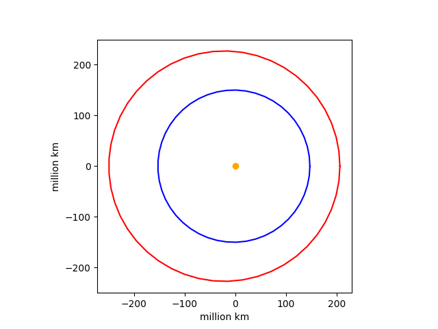
Kepler’s law says the square of a planet’s orbital period is proportional to the cube of the semi-major axis of its orbit. This means that increasing earth’s orbital period by 1 second would only require moving earth 3.16 km further from the sun.
***
[1] UTC stands for Universal Coordinated Time. From an earlier post,
The abbreviation UTC is an odd compromise. The French wanted to use the abbreviation TUC (temps universel coordonné) and the English wanted to use CUT (coordinated universal time). The compromise was UTC, which doesn’t actually abbreviate anything.
[2] In case you’re not familiar with the term “modest proposal,” it comes from the title of a satirical essay by Jonathan Swift. A modest proposal has come to mean an absurdly simple solution to a complex problem presented satirically.