The Laplace distribution is pointy in the middle and fat in the tails relative to the normal distribution.This post is about a probability distribution that is more pointy in the middle and fatter in the tails.
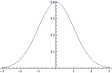
Here are pictures of the normal and Laplace (a.k.a. double exponential) distributions.
Normal:
Laplace:
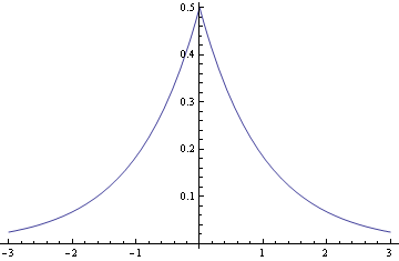
The normal density is proportional to exp(− x2/2) and the Laplace distribution is proportional to exp(-|x|). Near the origin, the normal density looks like 1 − x2/2 and the Laplace density looks like 1 − |x|. And as x gets large, the normal density goes to zero much faster than the Laplace.
Now let’s look at the distribution with density
f(x) = log(1 + 1/x²)
I don’t know a name for this. I asked on Cross Validated whether there was a name for this distribution and no knew of one. The density is related to the bounds on a density presented in this paper. Here’s a plot.
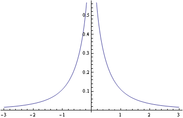
The density is unbounded near the origin, blowing up like −2 log( |x| ) as x approaches 0, and so is more pointed than the Laplace density. As x becomes large, log(1 + x−2) is asymptotically x−2 so the distribution has the same tail behavior as a Cauchy distribution, much heavier tailed than the Laplace density.
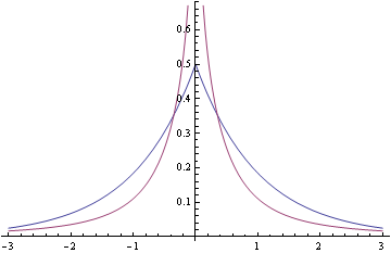
Here’s a plot of this new density and the Laplace density together to make the contrast more clear.
As William Huber pointed out in his answer on Cross Validated, this density has a closed-form CDF:
F(x) = 1/2 + (arctan(x) − x log( sin( arctan(x) ) ))/π
The paper mentioned above used a similar density as a Bayesian prior distribution in situations where many observations were expected to be small, though large values were expected as well.
What is the significance of a vertical asymptote in a probability distribution? What does it mean that the probability of x being 0 is infinitely large? I guess this can only apply to random variables that cannot take on the value 0?
The CDF must require Lebesgue integration – this isn’t Riemann integrable is it?
Dan: The probability isn’t infinite at zero, the probability density is infinite at zero. The density has to be integrated over a set to obtain a probability. It does mean that some small intervals can have high probability relative to their length, but this is a proper density: the total probably over the real line integrates to 1.
Riemann integration is adequate. You can integrate from -∞ to a and from b to ∞ and take the limits as a goes up to zero and b goes down to zero.
brilliant paper, FWIW; a follow-up showing relationships between shrinkage priors and Levy processes is at http://faculty.chicagobooth.edu/nicholas.polson/research/papers/Bayes1.pdf and well worth perusing.
Some distribution famili are infinite in zero
Cummulative F(x)=Tanh[x/p]^n has a zero asymptot when n<1
f(x) = (n/p)*(1-Tanh[x/p]^n) (x/p)^(n-1) and it is very useful in granulometric distribution.
The authors have a whole host of papers on arxiv along these lines, which I’d recommend for anyone interested in shrinkage in regression.
Another class of shrinkage priors, which are more analytically friendly than the horseshoe, are given in http://ftp.stat.duke.edu/WorkingPapers/10-08.html. The Laplace is a couple exponential pdf’s back to back; in that paper, the authors do the same with the Pareto.
Thanks for the interesting distribution. I have never seen a distribution function that had a vertical asymptote. I see how this integrates to one which is essential. Have you ever heard of a distribution function with a slant asymptote? I don’t think this could be possible because if the slant asymptote were not purely horizontal, it would fall asymptotically toward infinitity and negative infiinity as x approached infinity and negative infinity.
The distributions with vertical asymptotes I use most often are the gamma and beta.
The gamma distribution has a vertical asymptote at the origin for shape parameters less than 1. The beta distribution has a vertical asymptote at 0 if its first parameter is less than 1 and a vertical asymptote at 1 if its second parameter is less than 1.
This distribution looks very similar as a special case of the Generalized Asymmetric Laplace (GAL) as described by Kotz, Kozubowski and Podgorski (http://wolfweb.unr.edu/homepage/tkozubow/0_alm.pdf). Below you can find a link to a plot of the symmetric GAL with only one dimension:
http://tinypic.com/r/2wecenm/6
Just like the distribution John describes in his post, this distribution has a vertical asymptote at 0 (it’s location parameter). When one plots this special case of the GAL on the same plot as the distribution described by John, the differences become clear:
http://tinypic.com/r/36bti/6
That is: the distribution described by John is much more peaked an has fatter tails than the special case of the GAL.
I’ve been using the Laplace in the context of quantile regression or as shrinkage prior on regression coefficients. The distribution described by John could be used for the latter purpose too (as stated in the OP), but the Laplace has the advantage that it can be expressed as a scale mixture of normals (and makes efficient mcmc possible -> Gibbs sampling).
Thanks for your post!
Years ago, I came across a book on varites. It was an encyclopedia of distributions. I don’t recall the title/author and such.
I am missing something obvious in my sanity check of my understanding because f(1) = ln(2) or log10(2) that are both way larger than the plotted ~0.11.
I so want to understand all of it because it should result in a CDF that is the so-called cookie-cutter because I can introduce both a location and a scale.
My 2nd issue is that the F(x) needs an absolute value on the second arctan(x) according to the Excel interpretation.