My favorite numerical analysis book is Numerical Methods that Work. In the hardcover version of the book, the title was impressed in the cover and colored in silver letters. Before the last word of the title, there was another word impressed but not colored in. You had to look at the cover carefully to see that it actually says “Numerical methods that usually work.”
First published in 1970, the book’s specific references to computing power are amusingly dated. But book’s advice is timeless.
The chapter entitled “The care and treatment of singularities” gives several approaches for integrating functions that have a singularity. This post will elaborate on the simplest example from that chapter.
Suppose you want to compute the following integral.

The integrand is infinite at 0. There are a couple common hacks to get around this problem, and neither works well. One is simply to re-define the integrand so that it has some finite value at 0. That keeps the integration program from complaining about a division by zero, but it doesn’t help evaluate the integral accurately.
Another hack is to change the lower limit of integration from 0 to something a little larger. OK, but how much larger? And even if you replace 0 with something small, you still have the problem that your integrand is nearly singular near 0. Simple integration routines assume integrands are polynomial-like, and this integrand is not polynomial-like near zero.
The way to compute this integral is to subtract off the singularity. Since sin(x) is asymptotically equal to x as x goes to 0, √sin(x) is asymptotically √x. So if we subtract 1/√x, we’re left with a bounded integrand, and one that is considerably more polynomial-like than the one we started with. We then integrate by hand what we subtracted off. That is, we replace our original integral with the following pair of integrals.
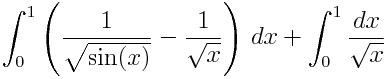
Compute the first numerically and the second analytically. Simpson’s rule with intervals of size 1/64 gives 0.03480535 for the first integral, which is correct to seven decimal places. The second integral is simply 2, so the total is 2.03480535.
Now lets look back at how our two hacks would have worked. Suppose we define our integrand f(x) to be 0 at x = 0. Then applying Simpson’s rule with step size 1/64 would give an integral of 3.8775, which is completely wrong. Bringing the step size down to 2^-20 makes things worse: the integral would then be 4.036. What if instead of defining the integrand to be 0 at 0, we define it to be some large value, say 10^6? In that case Simpson’s rule with step size 1/64 returns 5212.2 as the integral. Lowering the step size to 2^-20 improves the integral to 4.351, but still every figure is wrong since the integral is approximately 2.
What if we’d replaced 0 with 0.000001 and used Simpson’s rule on the original integral? That way we’d avoid the problem of having to define the integrand at 0. Then we’d have two sources of error. First the error from not integrating from 0 to 0.000001. That error is 0.002, which is perhaps larger than you’d expect: the change to the integral is 2000x larger than the change to the lower limit of integration. But this problem is insignificant compared to the next.
The more serious problem is applying Simpson’s rule to the integral even if we avoid 0 as the lower limit of integration. We still have a vertical asymptote, even if our limits of integration avoid the very singularity, and no polynomial ever had a vertical asymptote. With such decidedly non-polynomial behavior, we’d expect Simpsons rule and its ilk to perform poorly.
Indeed that’s what happens. With step size 1/64, Simpson’s rule gives a value of 9.086 for the integral, which is completely wrong since we know the integral is roughly 2.0348. Even with step size 2^-20, i.e. over a million function evaluations, Simpson’s rule gives 4.0328 for the integral.
Incidentally, if we had simply approximated our integrand 1/√sin(x) with 1/√x, we would have estimated the integral as 2.0 and been correct to two significant figures, while Simpson’s rule applied naively gets no correct figures. On the other hand, Simpson’s rule applied cleverly (i.e. by subtracting off the singularity) gives eight correct figures with little effort. As I concluded here, a crude method cleverly applied beats a clever technique crudely applied.

