Random inequalities I: introduction

Many Bayesian clinical trial methods have at their core a random inequality. Some examples from M. D. Anderson: adaptive randomization, binary safety monitoring, time-to-event safety monitoring. These method depends critically on evaluating P(X > Y) where X and Y are independent random variables. Roughly speaking, P(X > Y) is the probability that the treatment represented by X is better than the treatment represented by Y. In a trial with binary outcomes, X and Y may be the posterior probabilities of response on each treatment. In a trial with time-to-event outcomes, X and Y may be posterior probabilities of median survival time on two treatments.

People often have a little difficulty understanding what P(X > Y) means. What does it mean? If we take a sample from X and a random sample from Y, P(X >Y) is the probability that the former is larger than the latter. Most confusion around random inequalities comes from thinking of random variables as constants, not random quantities. Here are a couple examples.

First, suppose X and Y have normal distributions with standard deviation 1. If X has mean 4 and Y has mean 3, what is P(X > Y)? Some would say 1, because X is bigger than Y. But that’s not true. X has a larger mean than Y, but fairly often a sample from Y will be larger than a sample from X.  P(X > Y) = 0.76 in this case.

Next, suppose X and Y are identically distributed. Now what is P(X > Y)? I’ve heard people say zero because the two random variables are equal. But they’re not equal. Their distribution functions are equal but the two random variables are independent. P(X > y) = 1/2 by symmetry.

I believe there’s a psychological tendency to underestimate large inequality probabilities. (I’ve had several discussions with people who would not believe a reported inequality probability until they computed it themselves. These discussions are important when the decision whether to continue a clinical trial hinges on the result.) For example, suppose X and Y represent the probability of success in a trial in which there were 17 successes out of 30 on X and 12 successes out of 30 on Y. Using a beta distribution model, the density functions of X and Y are given below.

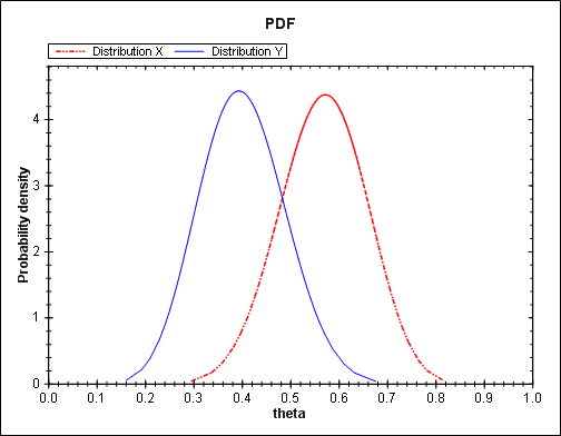
The density function for X is essentially the same as Y but shifted to the right. Clearly P(X > Y) is greater than 1/2. But how much greater than a half? You might think not too much since there’s a lot of mass in the overlap of the two densities. But P(X > Y) is a little more than 0.9.

The image above and the numerical results mentioned in this post were produced by the Inequality Calculator software.

Part II will discuss analytically evaluating random inequalities. Part III will discuss numerically evaluating random inequalities.