Introduction to Benford’s law
In 1881, Simon Newcomb noticed that the edges of the first pages in a book of logarithms were dirty while the edges of the later pages were clean. From this he concluded that people were far more likely to look up the logarithms of numbers with leading digit 1 than of those with leading digit 9. Frank Benford studied the same phenomena later and now the phenomena is known as Benford’s law, or sometime the Newcomb-Benford law.
A data set follows Benford’s law if the proportion of elements with leading digit d is approximately
log10((d + 1)/d).
You could replace “10” with b if you look at the leading digits in base b.
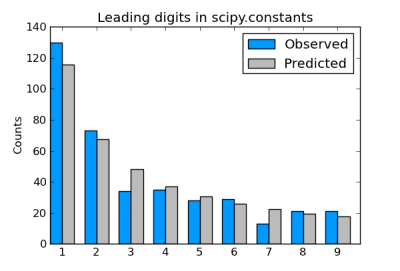
Sets of physical constants often satisfy Benford’s law, as I showed here for the constants defined in SciPy.
Incidentally, factorials satisfy Benford’s law exactly in the limit.
Weibull distributions
The Weibull distribution is a generalization of the exponential distribution. It’s a convenient distribution for survival analysis because it can have decreasing, constant, or increasing hazard, depending on whether the value of a shape parameter γ is less than, equal to, or greater than 1 respectively. The special case of constant hazard, shape γ = 1, corresponds to the exponential distribution.
Weibull and Benford
If the shape parameter of a Weibull distributions is “not too large” then samples from that distribution approximately follow Benford’s law (source). We’ll explore this statement with a little Python code.
SciPy doesn’t contain a Weibull distribution per se, but it does have support for a generalization of the Weibull known as the exponential Weibull. The latter has two shape parameters. We set the first of these to 1 to get the ordinary Weibull distribution.
      from math import log10, floor
      from scipy.stats import exponweib

      def leading_digit(x):
          y = log10(x) % 1
          return int(floor(10**y))

      def weibull_stats(gamma):

          distribution = exponweib(1, gamma)
          N = 10000
          samples = distribution.rvs(N)
          counts = [0]*10
          for s in samples:
              counts[ leading_digit(s) ] += 1

      print (counts)
Here’s how the leading digit distribution of a simulation of 10,000 samples from an exponential (Weibull with γ = 1) compares to the distribution predicted by Benford’s law.
      |---------------+----------+-----------|
      | Leading digit | Observed | Predicted |
      |---------------+----------+-----------|
      |             1 |     3286 |      3010 |
      |             2 |     1792 |      1761 |
      |             3 |     1158 |      1249 |
      |             4 |      851 |       969 |
      |             5 |      754 |       792 |
      |             6 |      624 |       669 |
      |             7 |      534 |       580 |
      |             8 |      508 |       511 |
      |             9 |      493 |       458 |
      |---------------+----------+-----------|
Looks like a fairly good fit. How could we quantify the fit so we can compare how the fit varies with the shape parameter? The most common approach is to use the chi-square goodness of fit test.
      def chisq_stat(O, E):
          return sum( (o - e)**2/e for (o, e) in zip(O, E) )
Here “O” stands for “observed” and “E” stands for “expected.” The observed counts are the counts we actually saw. The expected values are the values Benford’s law would predict:
expected = [N*log10((i+1)/i) for i in range(1, 10)]
Note that we don’t want to pass counts to chisq_stat but counts[1:] instead. This is because counts starts with 0 index, but leading digits can’t be 0 for positive samples.
Here are the chi square goodness of fit statistics for a few values of γ. (Smaller is better.)
      |-------+------------|
      | Shape | Chi-square |
      |-------+------------|
      |   0.1 |      1.415 |
      |   0.5 |      9.078 |
      |   1.0 |     69.776 |
      |   1.5 |    769.216 |
      |   2.0 |   1873.242 |
      |-------+------------|
This suggests that samples from a Weibull follow Benford’s law fairly well for shape γ < 1, i.e. for the case of decreasing hazard.