Nearly all the area of a high-dimensional sphere is near the equator. And by symmetry, it doesn’t matter which equator you take. Draw any great circle and nearly all of the area will be near that circle. This is the canonical example of “concentration of measure.”
What exactly do we mean by “nearly all the area” and “near the equator”? You get to decide. Pick your standard of “nearly all the area,” say 99%, and your definition of “near the equator,” say within 5 degrees. Then it’s always possible to take the dimension high enough that your standards are met. The more demanding your standard, the higher the dimension will need to be, but it’s always possible to pick the dimension high enough.
This result is hard to imagine. Maybe a simulation will help make it more believable.
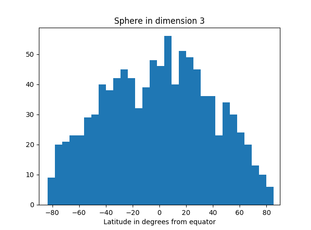
In the simulation below, we take as our “north pole” the point (1, 0, 0, 0, …, 0). We could pick any unit vector, but this choice is convenient. Our equator is the set of points orthogonal to the pole, i.e. that have first coordinate equal to zero. We draw points randomly from the sphere, compute their latitude (i.e. angle from the equator), and make a histogram of the results.
The area of our planet isn’t particularly concentrated near the equator.
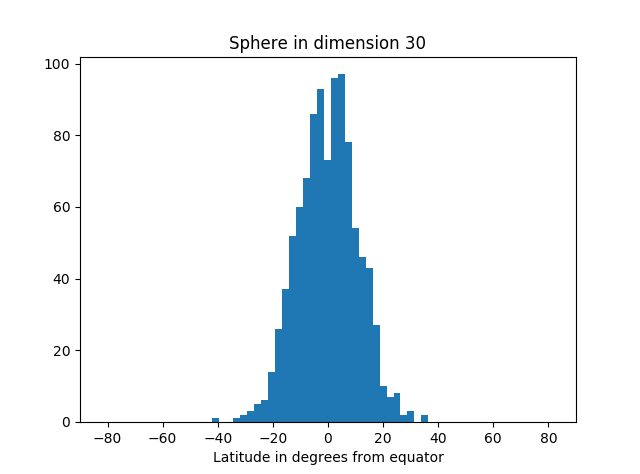
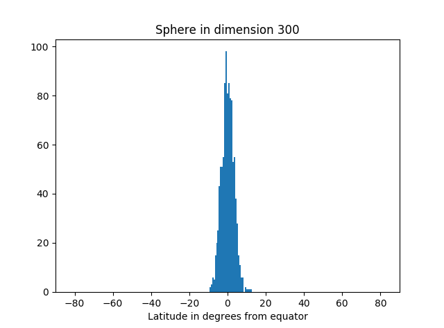
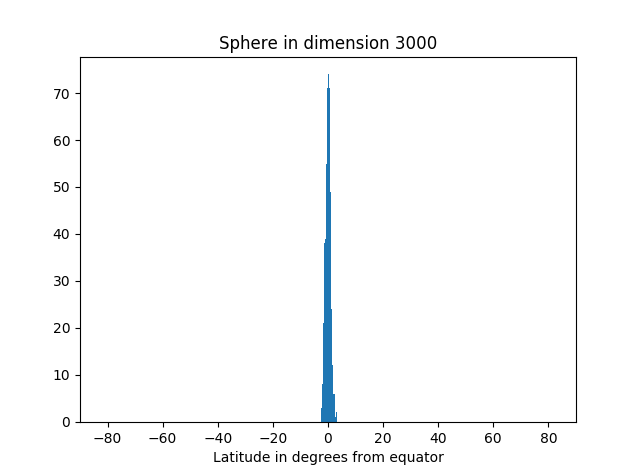
But as we increase the dimension, we see more and more of the simulation points are near the equator.
Here’s the code that produced the graphs.
from scipy.stats import norm
from math import sqrt, pi, acos, degrees
import matplotlib.pyplot as plt

def pt_on_sphere(n):
    # Return random point on unit sphere in R^n.
    # Generate n standard normals and normalize length.
    x = norm.rvs(0, 1, n)
    length = sqrt(sum(x**2))
    return x/length

def latitude(x):
    # Latitude relative to plane with first coordinate zero.
    angle_to_pole = acos(x[0]) # in radians
    latitude_from_equator = 0.5*pi - angle_to_pole
    return degrees( latitude_from_equator )

N = 1000 # number of samples

for n in [3, 30, 300, 3000]: # dimension of R^n

    latitudes = [latitude(pt_on_sphere(n)) for _ in range(N)]
    plt.hist(latitudes, bins=int(sqrt(N)))
    plt.xlabel("Latitude in degrees from equator")
    plt.title("Sphere in dimension {}".format(n))
    plt.xlim((-90, 90))
    plt.show()
Not only is most of the area near the equator, the amount of area outside a band around the equator decreases very rapidly as you move away from the band. You can see that from the histograms above. They look like a normal (Gaussian) distribution, and in fact we can make that more precise.
If A is a band around the equator containing at least half the area, then the proportion of the area a distance r or greater from A is bound by exp( −(n − 1)r² ). And in fact, this holds for any set A containing at least half the area; it doesn’t have to be a band around the equator, just any set of large measure.
Related post: Willie Sutton and the multivariate normal distribution
It wasn’t obvious to me why normalizing a vector of N+1 normal samples ends up being uniformly distributed over S^n. Might make an interesting post?
By “area”, we are talking about the measure of codimension 1, right? e.g. length in case of the 1-sphere and volume in the case of the 3-sphere.
This would be in contrast to, say, embedding a 2-sphere in higher dimensional space and asking about area.
@Jonathan: It’s not obvious if you think about taking N+1 samples from univariate normals, but it makes more sense if you think about taking one sample from a multivariate normal of dimension N+1. They turn out to be the same, thanks to the magic of Gaussian distributions. But the latter is obviously spherically symmetric since the density only depends on ||x||.
@roice: You could state everything in terms of intrinsic geometry — Riemann metrics and all that — not considering how the sphere is embedded in an ambient space. It doesn’t change the results, but the details are more complicated.
My question was more about whether we were talking about an (n-1)-dimensional “area” or 2-dimensional area. Rereading and looking at your code more closely, I think the answer is (n-1)-dimensional area.
> Pick your standard of “nearly all the area,” say 99%, and your definition of “near the equator,” say within 5 degrees. Then it’s always possible to take the dimension high enough that your standards are met. The more demanding your standard, the higher the dimension will need to be, but it’s always possible to pick the dimension high enough.
Here’s an easy proof of this using Markov’s inequality. First note that it’s enough to bound the orthogonal distance from the hyperplane describing the great circle, since the mapping from that distance to angle doesn’t depend on dimension.
Let u_1 be a unit normal vector for the hyperplane describing the great circle, and extend it to an orthonormal basis u_1,…,u_n. Let X be the random vector on the sphere.
Because X is on the sphere, we have (u_1^T X)^2 + … + (u_n^T X)^2 = 1. Taking expectations and using symmetry, E[(u_1^T X)^2] = 1/n.
Using Markov’s inequality, P[|u_1^T X| >= a] = P[(u_1^T X)^2 >= a^2] <= (1/n)/(a^2) = 1 / (n a^2). So for fixed a, we can bring this probability arbitrarily small be increasing n.
@John – Lovely argument from spherical symmetry. Thanks.
a similar observation, about those N-variate normal distributions, is that almost all of them are close to the sphere of size √N …. which might be the central limit theorem applied to Gamma distributions. Funny corollary: most Huge Data Sets will have lots of spurious correlations.
I don’t agree – choosing points on the sphere as projection of x=(x_i) with x_i normally distributed as you do, does not correspond to a uniform distribution over the sphere. (Check it out in 2D with the 1-sphere = unit circle : measure frequency of the angle phi in equally sized subintervals of [0,2pi] for your points x=[x[0],x[1]].)