Suppose you create a large matrix M by filling its components with random values. If M has size n by n, then we require the probability distribution for each entry to have mean 0 and variance 1/n. Then the Girko-Ginibri circular law says that the eigenvalues of M are approximately uniformly distributed in the unit disk in the complex plane. As the size n increases, the distribution converges to a uniform distribution on the unit disk.
The probability distribution need not be normal. It can be any distribution, shifted to have mean 0 and scaled to have variance 1/n, provided the tail of the distribution isn’t so thick that the variance doesn’t exist. If you don’t scale the variance to 1/n you still get a circle, just not a unit circle.
We’ll illustrate the circular law with a uniform distribution. The uniform distribution has mean 1/2 and variance 1/12, so we will subtract 1/2 and multiply each entry by √(12/n).
Here’s our Python code:
    import matplotlib.pyplot as plt
    import numpy as np

    n = 100
    M = np.random.random((n,n)) - 0.5
    M *= (12/n)**0.5
    w = np.linalg.eigvals(M)
    plt.scatter(np.real(w), np.imag(w))
    plt.axes().set_aspect(1)
    plt.show()
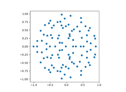
When n=100 we get the following plot.
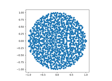
When n=1000 we can see the disk filling in more.
Note that the points are symmetric about the real axis. All the entries of M are real, so its characteristic polynomial has all real coefficients, and so its roots come in conjugate pairs. If we randomly generated complex entries for M we would not have such symmetry.
Related post: Fat-tailed random matrices
Circular low is fundamental in deep learning via spectral ergodicity, i.e., dynamics of weight matrices.
atan2(x,y) of two standard normal’s gives back the uniform distribution.