Symmetric Gaussian matrices
The previous post looked at the distribution of eigenvalues for very general random matrices. In this post we will look at the eigenvalues of matrices with more structure. Fill an n by n matrix A with values drawn from a standard normal distribution and let M be the average of A and its transpose, i.e. M = ½(A + AT). The eigenvalues will all be real because M is symmetric.
This is called a “Gaussian Orthogonal Ensemble” or GOE. The term is standard but a little misleading because such matrices may not be orthogonal.
Eigenvalue distribution
The joint probability distribution for the eigenvalues of M has three terms: a constant term that we will ignore, an exponential term, and a product term. (Source)
The exponential term is the same as in a multivariate normal distribution. This says the probability density drops of quickly as you go away from the origin, i.e. it’s rare for eigenvalues to be too big. The product term multiplies the distances between each pair of eigenvalues. This says it’s also rare for eigenvalues to be very close together.
(The missing constant to turn the expression above from a proportionality to an equation is whatever it has to be for the right side to integrate to 1. When trying to qualitatively understand a probability density, it usually helps to ignore proportionality constants. They are determined by the rest of the density expression, and they’re often complicated.)
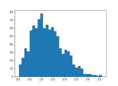
If eigenvalues are neither tightly clumped together, nor too far apart, we’d expect that the distance between them has a distribution with a hump away from zero, and a tail that decays quickly. We will demonstrate this with a simulation, then give an exact distribution.
Python simulation
The following Python code simulates 2 by 2 Gaussian matrices.
    import matplotlib.pyplot as plt
    import numpy as np

    n = 2
    reps = 1000

    diffs = np.zeros(reps)
    for r in range(reps):
        A = np.random.normal(scale=n**-0.5, size=(n,n))
        M = 0.5*(A + A.T)
        w = np.linalg.eigvalsh(M)
        diffs[r] = abs(w[1] - w[0])

    plt.hist(diffs, bins=int(reps**0.5))
    plt.show()
This produced the following histogram:

The exact probability distribution is p(s) = s exp(−s²/4)/2. This result is known as “Wigner’s surmise.”

There’s an interesting connection between the GOE and quantum chaotic spectra known as Bohigas-Giannoni-Schmit conjecture, http://www.scholarpedia.org/article/Bohigas-Giannoni-Schmit_conjecture .
In practice, the distribution of neighboring eigenvalues of systems’ Hamiltonians following the Wigner surmise (for certain classes of symmetries etc.) is often used as a signature of quantum chaos.
The problem has several generalizations that are also interesting. For an example, see the distribution of the (complex) eigenvalues of a random orthogonal matrix. For symmetric matrices, the distribution becomes more interesting when the values in an (n x n) are drawn from a nonnormal distribution such as U(0,1), although Wigner’s distribution still crops up for the nondominant eigenvalues! For some thoughts and graphs, see “The curious case of random eigenvalues.”
What if the values were drawn from an exponential distribution instead of standard normal?
This concrete example super helped me understand Wigner’s Surmise, but I would love to see it in N=3 because I have questions about how the diffs[r] = abs(w[1] – w[0]) operation works in this case? …so that I can be sure I understand the more generalized case.