Converting between quaternions and rotation matrices

In the previous post I wrote about representing rotations with quaternions. This representation has several advantages, such as making it clear how rotations compose. Rotations are often represented as matrices, and so it’s useful to be able to go between the two representations.

A unit-length quaternion (q0, q1, q2, q3) represents a rotation by an angle θ around an axis in the direction of (q1, q2, q3) where cos(θ/2) = q0. The corresponding rotation matrix is given below.

R = \begin{pmatrix} 2(q_0^2 + q_1^2) - 1 & 2(q_1 q_2 - q_0 q_3) & 2(q_1 q_3 + q_0 q_2) \\ 2(q_1 q_2 + q_0 q_3) & 2(q_0^2 + q_2^2) - 1 & 2(q_1 q_3 - q_0 q_1) \\ 2(q_1 q_3 - q_0 q_2) & 2(q_2 q_3 + q_0 q_1) & 2(q_0^2 + q_3^2) - 1 \end{pmatrix}

Going the other way around, inferring a quaternion representation from a rotation matrix, is harder. Here is a mathematically correct but numerically suboptimal method known [1] as the Chiaverini-Siciliano method.

\begin{align*} q_0 &= \frac{1}{2} \sqrt{1 + r_{11} + r_{22} + r_{33}} \\ q_1 &= \frac{1}{2} \sqrt{1 + r_{11} - r_{22} - r_{33}} \text{ sgn}(r_{32} - r_{32}) \\ q_2 &= \frac{1}{2} \sqrt{1 - r_{11} + r_{22} - r_{33}} \text{ sgn}(r_{13} - r_{31}) \\ q_3 &= \frac{1}{2} \sqrt{1 - r_{11} - r_{22} + r_{33}} \text{ sgn}(r_{21} - r_{12}) \end{align*}

Here sgn is the sign function; sgn(x) equals 1 if x is positive and −1 if x is negative. Note that the components only depend on the diagonal of the rotation matrix, aside from the sign terms. Better numerical algorithms make more use of the off-diagonal elements.

Accounting for degrees of freedom

Something seems a little suspicious here. Quaternions contain four real numbers, and 3 by 3 matrices contain nine. How can four numbers determine nine numbers? And going the other way, out of the nine, we essentially choose three that determine the four components of a quaternion.

Quaterions have four degrees of freedom, but we’re using unit quaternions, so there are basically three degrees of freedom. Likewise orthogonal matrices have three degrees of freedom. An axis of rotation is a point on a sphere, so that has two degrees of freedom, and the degree of rotation is the third degree of freedom.

In topological terms, the unit quaternions and the set of 3 by 3 orthogonal matrices are both three dimensional manifolds, and the former is a double cover of the latter. It is a double cover because a unit quaternion q corresponds to the same rotation as −q.

Python code

Implementing the equations above is straightforward.

import numpy as np

def quaternion_to_rotation_matrix(q):
    q0, q1, q2, q3 = q
    return np.array([
        [2*(q0**2 + q1**2) - 1, 2*(q1*q2 - q0*q3), 2*(q1*q3 + q0*q2)],
        [2*(q1*q2 + q0*q3), 2*(q0**2 + q2**2) - 1, 2*(q2*q3 - q0*q1)],
        [2*(q1*q3 - q0*q2), 2*(q2*q3 + q0*q1), 2*(q0**2 + q3**2) - 1]
    ]) 

def rotation_matrix_to_quaternion(R):
    r11, r12, r13 = R[0, 0], R[0, 1], R[0, 2]
    r21, r22, r23 = R[1, 0], R[1, 1], R[1, 2]
    r31, r32, r33 = R[2, 0], R[2, 1], R[2, 2]
    
    # Calculate quaternion components
    q0 = 0.5 * np.sqrt(1 + r11 + r22 + r33)
    q1 = 0.5 * np.sqrt(1 + r11 - r22 - r33) * np.sign(r32 - r23)
    q2 = 0.5 * np.sqrt(1 - r11 + r22 - r33) * np.sign(r13 - r31)
    q3 = 0.5 * np.sqrt(1 - r11 - r22 + r33) * np.sign(r21 - r12)
    
    return np.array([q0, q1, q2, q3])

Random testing

We’d like to test the code above by generating random quaternions, converting the quaternions to rotation matrices, then back to quaternions to verify that the round trip puts us back essentially where we started. Then we’d like to go the other way around, starting with randomly generated rotation matrices.

To generate a random unit quaternion, we generate a vector of four independent normal random values, then normalize by dividing by its length. (See this recent post.)

To generate a random rotation matrix, we use a generator that is part of SciPy.

Here’s the test code:

def randomq():
    q = norm.rvs(size=4)
    return q/np.linalg.norm(q)

def randomR():
    return special_ortho_group.rvs(dim=3)

np.random.seed(20250507)
N = 10

for _ in range(N):
    q = randomq()
    R = quaternion_to_rotation_matrix(q)
    t = rotation_matrix_to_quaternion(R)
    print(np.linalg.norm(q - t))
    
for _ in range(N):
    R = randomR()
    q = rotation_matrix_to_quaternion(R)
    T = quaternion_to_rotation_matrix(q)
    print(np.linalg.norm(R - T))

The first test utterly fails, returning six 2s, i.e. the round trip vector is as far as possible from the vector we started with. How could that happen? It must be returning the negative of the original vector. Now go back to the discussion above about double covers: q and −q correspond to the same rotation.

If we go back and add the line

    q *= np.sign(q[0])

then we standardize our random vectors to have a positive first component, just like the vectors returned by rotation_matrix_to_quaternion.

Now our tests all return norms on the order of 10−16 to 10−14. There’s a little room to improve the accuracy, but the results are good.

Update: I did some more random testing, and found errors on the order of 10−10. Then I was able to create a test case where rotation_matrix_to_quaternion threw an exception because one of the square roots had a negative argument. In [1] the authors get around this problem by evaluating two theoretically equivalent expressions for each of the square root arguments. The expressions are complementary in the sense that both should not lead to numerical difficulties at the same time.

[1] See “Accurate Computation of Quaternions from Rotation Matrices” by Soheil Sarabandi and Federico Thomas for a better numerical algorithm. See also the article “A Survey on the Computation of Quaternions From Rotation Matrices” by the same authors.

A better integral for the normal distribution

For a standard normal random variable Z, the probability that Z exceeds some cutoff z is given by

\mbox{Prob}(Z \geq z) = Q(z) = \frac{1}{\sqrt{2\pi}} \int_z^\infty \exp(-x^2/2)\, dx

If you wanted to compute this probability numerically, you could obviously evaluate its defining integral numerically. But as is often the case in numerical analysis, the most obvious approach is not the best approach. The range of integration is unbounded and it varies with the argument.

J. W. Craig [1] came up with a better integral representation, better from the perspective of numerical integration. The integration is always over the same finite interval, with the argument appearing inside the integrand. The integrand is smooth and bounded, well suited to numerical integration.

For positive z, Craig’s integer representation is

Q(z) = \frac{1}{\pi} \int_0^{\pi/2} \exp\left( -\frac{z^2}{2\sin^2 \theta} \right) \, d\theta

Illustration

To show that the Craig’s integral is easy to integrate numerically, we’ll evaluate it using Gaussian quadrature with only 10 integration points.

    from numpy import sin, exp, pi
    from scipy import integrate
    from scipy.stats import norm

    for x in [0.5, 2, 5]:
        q, _ = integrate.fixed_quad(
            lambda t: exp(-x**2 / (2*sin(t)**2))/pi,
            0.0, pi/2, n=10)
        print(q, norm.sf(x))

(SciPy uses sf (“survival function”) for the CCDF. More on that here.)

The code above produces the following.

    0.30858301 0.30853754
    0.02274966 0.02275013
    2.86638437e-07 2.86651572e-07

So with 10 integration points, we get four correct figures. And the accuracy seems to be consistent for small, medium, and large values of x. (Five standard deviations is pretty far out in the tail of a normal distribution, as evidenced by the small value of the integral.)

Related posts

[1] J. W. Craig, A new, simple and exact result for calculating the probability of error for two-dimensional signal constellations, in TEEE MILCOM’91 Conf. Rec., Boston, MA (1991) рр. 25.2.1-25.5.5.

Computing inverse factorial

I needed the inverse factorial function for my previous post. I was sure I’d written a post on computing the inverse factorial, and intended to reuse the code from that earlier post. But when I searched I couldn’t find anything, so I’m posting the code here for my future reference and for anyone else who may need it.

Given a positive number x, how can you find a number n such that n! = x, or such that n! ≈ x?

Mathematical software tends to work with the gamma function rather than factorials because Γ(x) extends x! to real numbers, with the relation Γ(x+1) = x!. The left side is often taken as a definition of the right side when x is not a positive integer.

Not only do we prefer to work with the gamma function, it’s easier to work with the logarithm of the gamma function to avoid overflow.

The Python code below finds the inverse of the log of the gamma function using the bisection method. This method requires an upper and lower bound. If we only pass in positive values, 0 serves as a lower bound. We can find an upper bound by trying powers of 2 until we get something large enough.

from scipy.special import gammaln
from scipy.optimize import bisect

def inverse_log_gamma(logarg):
    assert(logarg > 0)
    a = 1
    b = 2
    while b < logarg:
        b = b*2
    return bisect(lambda x: gammaln(x) - logarg, a, b)

def inverse_factorial(logarg):
    g = inverse_log_gamma(logarg)
    return round(g)-1 

Note that the inverse_factorial function takes the logarithm of the value whose inverse factorial you want to compute.

For example,

inverse_factorial(log(factorial(42))))

returns 42.

Working on the log scale lets us work with much larger numbers. The factorial of 171 is larger than the largest IEEE double precision number, and so inverse_factorial could not return any value larger than 171 if we passed in x rather than log x. But by taking log x as the argument, we can calculate inverse factorials of numbers so large that the factorial overflows.

For example, suppose we want to find the value of m such that m! is the closest factorial to √(2024!), as we did in the previous post. We can use the code

inverse_factorial(gammaln(2025)/2)

to find m = 1112 even though 1112! is on the order of 102906, far larger than the largest representable floating point number, which is on the order of 10308.

When n! = x does not have an exact solution, there is some choice over what value of n to return as the inverse factorial of x. The code above minimizes the distance from n! to x on a log scale. You might want to modify the code to minimize the distance on a linear scale, or to find the largest n with n! < x, or the smallest n with n! > x depending on your application.

Related posts

Numerical integral with a singularity

Richard Hamming [1] gives this nice example of an integral with a mild singularity:

\int_0^1 \log(\sin(x))\, dx

The integrand approaches −∞ as x approaches 0 and yet the integral is finite. If we try into numerically evaluate this integral, we will either get inaccurate results or we will have to go to a lot of work.

This post will show that with a clever reformulation of the problem we use simple methods to get accurate results, or use sophisticated methods with fewer function evaluations.

As I wrote about years ago, a common technique for dealing with singularities is to add and subtract a function with the same asymptotic behavior that can be integrated by hand. Hamming does a slight variation on this, multiplying and dividing by x inside the logarithm.

\begin{align*} \int_0^1 \log(\sin(x))\, dx &= \int_0^1 \log(x)\, dx + \int_0^1 \log\left(\frac{\sin(x)}{x}\right) \, dx \\ &=  -1 + \int_0^1 \log\left(\frac{\sin(x)}{x}\right) \, dx \end{align*}

Here we integrated the singular part, log(x), and we are left with numerically integrating a well-behaved function, one that is smooth and bounded on the interval of integration. Because sin(x) ≈ x for small x, we can define sin(x)/x to be 1 at 0 and have a smooth function.

We’ll use NumPy’s sinc function to handle sin(x)/x properly near 0. There are two conventions for defining the sinc function, either as sin(x)/x or as sin(πx)/πx. NumPy uses the latter convention, so we define our own sinc function as follows.

import numpy as np
def mysinc(x): return np.sinc(x/np.pi)

Trapezoid rule

Let’s use the simplest numerical method, the trapezoid rule.

We run into a problem immediately: if we chop up the interval [0, 1] in a way that puts an integration point at 0, our resulting integral will be infinite. We could replace 0 with some ε > 0, but if we do, we should try a few different values of ε to see whether our choice of ε greatly impacts our integral.

for ε in [1e-6, 1e-7, 1e-8]:
    xs = np.linspace(ε, 1, 100)
    integral = sum( np.log(np.sin(x)) for x in xs ) / 100

This gives us

-1.152996659484881
-1.1760261818509377
-1.1990523999312201

suggesting that the integral does indeed depend on ε. We’ll see soon that our integral evaluates to around −1.05. So our results are not accurate, and the smaller ε is, the worse our answer is. [2]

Now let’s evaluate the integral as Hamming suggests. We’ll use a varying number of integration points so the difference between our integral estimates will give us some idea whether we’re converging.

for N in [25, 50, 100]:
    xs = np.linspace(0, 1, N)
    integral = sum( np.log(mysinc(xs)) )/N
    integral -= 1 # subtract the integral of log(x)
    print(integral)

This gives us

-1.0579531812873197
-1.057324013010989
-1.057019035348765

The consistency between the result suggests the integral is around −1.057.

Adaptive integration

We said at the top of this article that Hamming’s reformulation would either let us get accurate results from simple methods or let us get by with fewer function evaluations using a sophisticated method. Now we’ll demonstrate the latter, using the adaptive integration algorithm quad from SciPy.

from scipy.integrate import quad

# Integrate log(sin(x)) from 0 to 1
integral, error = quad(lambda x: np.log(np.sin(x)), 0, 1)
print(integral, error) 

# Integrate log(x sin(x)/x) = log(x) + log(mysinc(x)) from 0 to 1
integral, error = quad(lambda x: np.log(mysinc(x)), 0, 1)
integral -= 1
print(integral, error)

This prints

-1.0567202059915843 1.7763568394002505e-15
-1.056720205991585 6.297207865333937e-16

suggesting that both approaches are working. Both estimate their error to be near machine precision. But as we’ll see, the direct approach uses about 10 times as many function evaluations.

Let’s ask quad to return more details by adding full_output = 1 as an argument.

integral, error, info = quad(lambda x: np.log(np.sin(x)), 0, 1, full_output=1)
print(integral, error, info["neval"])

integral, error, info = quad(lambda x: np.log(mysinc(x)), 0, 1, full_output=1)
integral -= 1
print(integral, error, info["neval"])

This shows that the first integration used 231 function evaluations, but the second used only 21.

The difference in efficiency doesn’t matter when you’re evaluating an integral one time, but if you were repeatedly evaluating similar integrals inside a loop, subtracting off the singularity could make your problem run 10 times faster. Simulations involving Bayesian statistics can have such integrations in the inner loop, and so making an integration an order of magnitude faster could make the overall simulation an order of magnitude faster, reducing CPU-days to CPU-hours.

Related posts

[1] Richard Hamming, Numerical Methods for Scientists and Engineers. Second edition. Dover.

[2] We can get better results if we let ε and 1/N go to zero at the same rate. The following code produces mediocre results, but better results than above.

for N in [10, 100, 1000]:
    xs = np.linspace(1/N, 1, N)
    integral = sum( np.log(np.sin(x)) for x in xs ) / N
    print(integral)

This prints

-0.8577924592777062
-1.0253626377143321
-1.05243363818431

which at least seems to be getting closer to the correct result, but has bad accuracy for so many function evaluations.

Equation of an ellipse or hyperbola through five points

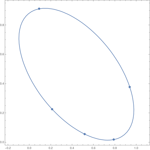
Yesterday I wrote about the equation of a circle through three points. This post will be similar, looking at the equation of an ellipse or hyperbola through five points. As with the earlier post, we can write down an elegant equation right away. Making the equation practical will take more work.

The equation of a general conic section through five points

\begin{vmatrix} x^2 & y^2 & xy & x & y & 1 \\ x_1^2 & y_1^2 & x_1 y_1 & x_1 & y_1 & 1 \\ x_2^2 & y_2^2 & x_2 y_2 & x_2 & y_2 & 1 \\ x_3^2 & y_3^2 & x_3 y_3 & x_3 & y_3 & 1 \\ x_4^2 & y_4^2 & x_4 y_4 & x_4 & y_4 & 1 \\ x_5^2 & y_5^2 & x_5 y_5 & x_5 & y_5 & 1 \\ \end{vmatrix} = 0

Direct but inefficient solution

The most direct (though not the most efficient) way to turn this into an equation

Ax^2 + By^2 + Cxy + Dx + Ey + F = 0

is to expand the determinant by minors of the first row.

A = \begin{vmatrix} y_1^2 & x_1 y_1 & x_1 & y_1 & 1 \\ y_2^2 & x_2 y_2 & x_2 & y_2 & 1 \\ y_3^2 & x_3 y_3 & x_3 & y_3 & 1 \\ y_4^2 & x_4 y_4 & x_4 & y_4 & 1 \\ y_5^2 & x_5 y_5 & x_5 & y_5 & 1 \\ \end{vmatrix} ,\, B = - \begin{vmatrix} x_1^2 & x_1 y_1 & x_1 & y_1 & 1 \\ x_2^2 & x_2 y_2 & x_2 & y_2 & 1 \\ x_3^2 & x_3 y_3 & x_3 & y_3 & 1 \\ x_4^2 & x_4 y_4 & x_4 & y_4 & 1 \\ x_5^2 & x_5 y_5 & x_5 & y_5 & 1 \\ \end{vmatrix}

C = \begin{vmatrix} x_1^2 & y_1^2 & x_1 & y_1 & 1 \\ x_2^2 & y_2^2 & x_2 & y_2 & 1 \\ x_3^2 & y_3^2 & x_3 & y_3 & 1 \\ x_4^2 & y_4^2 & x_4 & y_4 & 1 \\ x_5^2 & y_5^2 & x_5 & y_5 & 1 \\ \end{vmatrix} ,\, D = - \begin{vmatrix} x_1^2 & y_1^2 & x_1 y_1 & y_1 & 1 \\ x_2^2 & y_2^2 & x_2 y_2 & y_2 & 1 \\ x_3^2 & y_3^2 & x_3 y_3 & y_3 & 1 \\ x_4^2 & y_4^2 & x_4 y_4 & y_4 & 1 \\ x_5^2 & y_5^2 & x_5 y_5 & y_5 & 1 \\ \end{vmatrix}

 E = \begin{vmatrix} x_1^2 & y_1^2 & x_1 y_1 & x_1 & 1 \\ x_2^2 & y_2^2 & x_2 y_2 & x_2 & 1 \\ x_3^2 & y_3^2 & x_3 y_3 & x_3 & 1 \\ x_4^2 & y_4^2 & x_4 y_4 & x_4 & 1 \\ x_5^2 & y_5^2 & x_5 y_5 & x_5 & 1 \\ \end{vmatrix} ,\, F = - \begin{vmatrix} x_1^2 & y_1^2 & x_1 y_1 & x_1 & y_1\\ x_2^2 & y_2^2 & x_2 y_2 & x_2 & y_2\\ x_3^2 & y_3^2 & x_3 y_3 & x_3 & y_3\\ x_4^2 & y_4^2 & x_4 y_4 & x_4 & y_4\\ x_5^2 & y_5^2 & x_5 y_5 & x_5 & y_5\\ \end{vmatrix}

More efficient solution

It would be much more efficient to solve a system of equations for the coefficients. Since the determinant at the top of the page is zero, the columns are linearly dependent, and some linear combination of those columns equals the zero vector. In fact, the coefficients of such a linear combination are the coefficients A through F that we’re looking for.

We have an unneeded degree of freedom since any multiple of the coefficients is valid. If we divide every coefficient by A, then the new leading coefficient is 1. This gives us five equations in five unknowns.

\begin{bmatrix} y_1^2 & x_1 y_1 & x_1 & y_1 & 1 \\ y_2^2 & x_2 y_2 & x_2 & y_2 & 1 \\ y_3^2 & x_3 y_3 & x_3 & y_3 & 1 \\ y_4^2 & x_4 y_4 & x_4 & y_4 & 1 \\ y_5^2 & x_5 y_5 & x_5 & y_5 & 1 \\ \end{bmatrix} \begin{bmatrix} B \\ C \\ D \\ E \\ F \\ \end{bmatrix} = - \begin{bmatrix} x_1^2 \\ x_2^2 \\ x_3^2 \\ x_4^2 \\ x_5^2 \\ \end{bmatrix}

Python example

The following code will generate five points and set up the system of equations Ms = b whose solution s will give our coefficients.

    import numpy as np

    np.random.seed(20230619)

    M = np.zeros((5,5))
    b = np.zeros(5)
    for i in range(5):
        x = np.random.random()
        y = np.random.random()    
        M[i, 0] = y**2
        M[i, 1] = x*y
        M[i, 2] = x
        M[i, 3] = y
        M[i, 4] = 1
        b[i] = -x*x

Now we solve for the coefficients.

    s = np.linalg.solve(M, b)
    A, B, C, D, E, F = 1, s[0], s[1], s[2], s[3], s[4]

Next we verify that the points we generated indeed lie on the conic section whose equation we just found.

    for i in range(5):
        x = M[i, 2]
        y = M[i, 3]
        assert( abs(A*x*x + B*y*y + C*x*y + D*x + E*y + F) < 1e-10 )

Ellipse or hyperbola?

It turns out that the five points generated above lie on a hyperbola.

If we had set the random number generator seed to 20230620 we would have gotten an ellipse.

When we generate points at random, as we did above, we will almost certainly get an ellipse or a hyperbola. Since we’re generating pseudorandom numbers, there is some extremely small chance the generated points would lie on a line or on a parabola. In theory, this almost never happens, in the technical sense of “almost never.”

If 4ABC² is positive we have a an ellipse. If it is negative we have a hyperbola. If it is zero, we have a parabola.

Related posts

AM over GM

Suppose you take the arithmetic mean and the geometric mean of the first n integers. The ratio of these two means converges to e/2 as n grows [1]. In symbols,

\lim_{n\to\infty} \frac{(1 + 2 + 3 + \cdots + n)/n}{\sqrt[n]{1 \cdot2 \cdot3 \cdots n}} = \frac{e}{2}

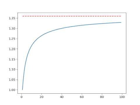
Now suppose we wanted to visualize the convergence by plotting the expression on the left side for a sequence of ns.

First let’s let n run from 1 to 100.

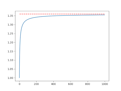
This isn’t very convincing. Maybe the convergence is just slow, or maybe it’s not actually converging to e/2. Let’s make another plot including larger values of n. This will require a little additional work.

Avoiding overflow

Here’s the code that made the plot above.

    import matplotlib.pyplot as plt
    import numpy as np
    from scipy.special import factorial

    AM = lambda n: (n+1)/2
    GM = lambda n: factorial(n)**(1/n)
    n = np.arange(1, 100)
    plt.plot(n, AM(n)/GM(n))
    plt.plot(n, 0*n + np.exp(1)/2, 'r--')

This works for n up to 170, but it fails when n = 171 because at that point factorial overflows.

This is a very common situation. We ultimately want to compute a fairly small number, but we encounter extremely large numbers in an intermediate step.

We need to avoid directly calculating n! before taking the nth root. The way to do this is to work with logarithms. Now n! = Γ(n+1) and SciPy has a function for computing the log of the gamma function directly without first computing the gamma function, thus avoiding overflow.

We replace GM above with GM2 below:

    GM2 = lambda n: np.exp(gammaln(n+1)/n)

Now we compute the geometric mean of the first n natural numbers for very large values of n. We only need n = 1000 to see convergence, but the code could handle much larger values of n without overflowing.

Related posts

[1] Richard P. Kubelka. Means to an End. Mathematics Magazine, Vol. 74, No. 2 (April 2001), pp. 141–142

Solve for Jacobi sn parameter to have given period(s)

Here’s a calculation that I’ve had to do a few times. I’m writing it up here for my future reference and for the benefit of anybody else who needs to do the same calculation.

The Jacobi sn function is doubly periodic: it has one period as you move along the real axis and another period as you move along the imaginary axis. Its values are determined by a fundamental rectangle, and here we solve for a parameter 0 ≤ m < 1 that yields a desired length, or width, or aspect ratio for this rectangle.

You cannot specify both the length and width of the fundamental rectangle independently: you only have one degree of freedom. You can specify its length, or width, or aspect ratio.

This post focuses on sn, then explains how to modify the results for the other Jacobi elliptic functions—cn, dn, sc, etc.—at the end.

Given period

A parameter value m corresponds to a horizontal period of 4K(m) and a vertical period of 2K(1-m) where K is the complete elliptic integral of the first kind.

K(m) is an increasing function from [0, 1) to [π/2, ∞). So the minimum horizontal period is 2π and the minimum vertical period is π.

Given aspect ratio

The ratio of the horizontal period to the vertical period is given by

r(m) = 4K(m) / 2K(1−m) = 2K(m) / K(1−m).

The function r is an increasing function from [0, 1) to [0, ∞), so any aspect ratio is possible. This is important, for example, in conformal mapping. You cannot specify the length and width of the fundamental period independently, but you can solve for the parameter m that gives the aspect ratio you want, then follow it by a dilation to then get the length and width you want.

Numerical computation

If you need to find m efficiently or to high precision, see [1]. The code here simple and good enough for my purposes, and hopefully good enough for yours.

We need to either invert K or r, both of which are monotone functions, and so we can use the bisection method to find the value of m we’re after. The bisection method is not the most efficient, but it’s simple and very robust.

Python code

    from numpy import pi, linspace
    from scipy.special import ellipk, ellipj
    from scipy.optimize import bisect
    
    def invert_ellipk(K):
        "Given K, find m such that K(m) = K."
        assert(K >= pi/2)
        if K == pi/2:
            return 0
    
        # Find a bracket [a, b] for m
        a = 0
        b = 0.5
        y = ellipk(b)
        while y < K:
            b = 0.5*(b + 1)
            y = ellipk(b)
        return bisect(lambda m: ellipk(m)-K, a, b)
    
    def invert_horizontal_period(T):
        "Find parameter m such that sn(z, m) has real period T."
        return invert_ellipk(T/4)
    
    def invert_vertical_period(T):
        "Find parameter m such that sn(z, m) has imaginary period T."    
        return invert_ellipk(T/2)
    
    def invert_r(r):
        "Find parameter m such that the fundamental rectangle of sn(z, m) has aspect ratio r."
    
        ratio = lambda m: 2*ellipk(m)/ellipk(1-m)
        
        if r == 2:
            return 1/2
    
        a, b = 0.5, 0.5
        while ratio(b) < r: b = 0.5*(1 + b) while ratio(a) > r:
            a /= 2
        return bisect(lambda m: r - ratio(m), a, b)

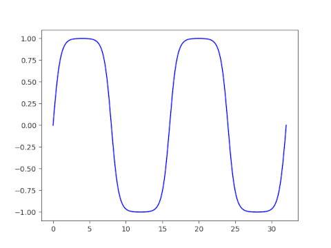
To test the code, let’s find m such that sn(z, m) has period 5 along the real axis.

    import matplotlib.pyplot as plt

    T = 16
    m = invert_horizontal_period(T)
    print(4*ellipk(m))
    assert(abs(4*ellipk(m) - T) < 1e-8)
    x = linspace(0, 2*T, 200)
    plt.plot(x, sn(x, m))

This produces a plot that does have period 16.

Other Jacobi elliptic functions

There are 12 Jacobi elliptic functions, denoted with all pairs of {s, c, d, n} such that the two letters are different. The periods of the functions fall into three groups.

The functions sn, ns, cd, and dc all have real period 4K(m) and imaginary period 2K(1-m).

The functions cn, nc, ds, and sd all have real period 4K(m) and imaginary period 4K(1-m).

The functions cs, sc, dn, and nd all have real period 2K(m) and imaginary period 4K(1-m).

You can find plots of fundamental rectangles of these 12 functions here.

[1] Toshio Fukushima. Numerical computation of inverse complete elliptic integrals of the first and second kinds. Journal of Computational and Applied Mathematics. 249 (2013) 37–50.


Logarithmic spiral

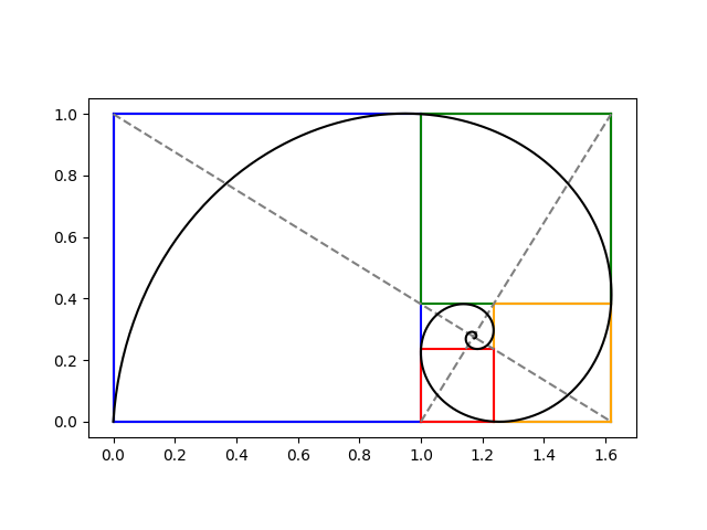
I’ve seen an image similar to the following many times, but I don’t recall any source going into detail regarding how the spiral is constructed. This post will do just that.

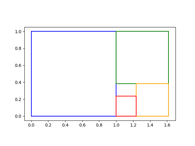
The previous post constructed iterated golden rectangles. We start with a golden rectangle and imagine chopping of first the blue, then the green, then the orange, and then the red square. We could continue this process on the inner most rectangle, over and over.

At this point, many sources would say “Hey look! We can draw a spiral that goes through two corners of each square” without explicitly stating an equation for the spiral. We’ll find spiral, making everything explicit.

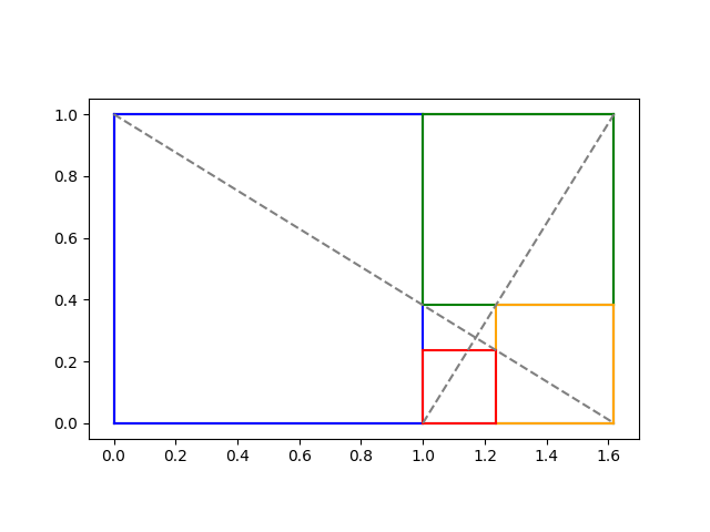
In the previous post we showed how to find the limit of the iterative process at the intersection of the two diagonal lines below.

We showed that the intersection is at

x0 = (2φ + 1)/(φ + 2)

and

y0 = 1/(φ + 2).

Logarithmic spirals

A logarithmic spiral centered at the origin has the polar equation

r(θ) = a exp(kθ)

for some constants a and k. Our spiral will be such a spiral shifted to center at (x0y0).

Imagine a spiral going from the lower left to the top left of the blue square, then to the top left of the green square, then to the top right of the orange square etc., passing through two corners of every square. Every time θ goes through a quarter turn, i.e. π/2 radians, our rectangles get smaller by a factor of φ. We can use this to solve for k because

a exp(k(θ + π/2)) = φ a exp()

and so

exp(kπ/2) = φ

and

k = 2log(φ) / π.

To summarize what we know so far, if we shift our spiral to the origin, it has equation in polar form

r(θ) = a exp(kθ)

where we now know k but don’t yet know a.

Finding θ and a

To get our actual spiral, we have to shift the origin to (x0, y0) which we have calculated above. Converting from polar to rectangular coordinates so we can do the shift, we have

x(θ) = x0 + a exp(kθ) cos(θ)

y(θ) = y0 + a exp(kθ) sin(θ)

We can find the parameter a by knowing that our spiral passes through the origin, the bottom left corner in the plots above. At what value of θ does the curve go through the origin? We have a choice; values of θ that differ by multiples of 2π will give different values of a.

The angle θ is the angle made by the line connecting (0, 0) to (x0, y0). We can find θ via

θ0 = atan2(−y0, −x0).

Here’s Python code to find θ0:

    import numpy as np

    phi = (1 + 5**0.5)/2
    y0 = 1/(2+phi)
    x0 = (2*phi + 1)*y0
    theta0 = np.arctan2(-y0, -x0)

Then we solve for a from the equation x0) = 0.

    k = 2*np.log(phi)/np.pi
    a = -x0 / (np.exp(k*theta0)*np.cos(theta0)))

Plots

Now we have all the parameters we need to define our logarithmic spiral. The following code draws our logarithmic spiral on top of the plot of the rectangles.

    t = np.linspace(-20, theta0, 1000)
    def x(t): return x0 + a*np.exp(k*t)*np.cos(t)
    def y(t): return y0 + a*np.exp(k*t)*np.sin(t)
    plt.plot(x(t), y(t), "k-")

The result is the image at the top of the post.

Find log normal parameters for given mean and variance

Earlier today I needed to solve for log normal parameters that yield a given mean and variance. I’m going to save the calculation here in case I needed in the future or in case a reader needs it. The derivation is simple, but in the heat of the moment I’d rather look it up and keep going with my train of thought.

NB: The parameters μ and σ² of a log normal distribution are not the mean and variance of the distribution; they are the mean and variance of its log.

If m is the mean and v is the variance then

\begin{align*} m &= \exp(\mu + \sigma^2/2) \\ v &= (\exp(\sigma^2) - 1) \exp(2\mu + \sigma^2) \end{align*}

Notice that the square of the m term matches the second part of the v term.

Then

\frac{v}{m^2} = \exp(\sigma^2) -1

and so

\sigma^2 = \log\left(\frac{v}{m^2} + 1 \right)

and once you have σ² you can find μ by

\mu = \log m - \sigma^2/2

Here’s Python code to implement the above.

    from numpy immport log
    def solve_for_log_normal_parameters(mean, variance):
        sigma2 = log(variance/mean**2 + 1)
        mu = log(mean) - sigma2/2
        return (mu, sigma2)

And here’s a little test code for the code above.

    mean = 3.4
    variance = 5.6

    mu, sigma2 = solve_for_log_normal_parameters(mean, variance)

    X = lognorm(scale=exp(mu), s=sigma2**0.5)
    assert(abs(mean - X.mean()) < 1e-10)
    assert(abs(variance - X.var()) < 1e-10)

Related posts

Finding Lagrange points L1 and L2

The James Webb Space Telescope (JWST) is on its way to the Lagrange point L2 of the Sun-Earth system. Objects in this location will orbit the Sun at a fixed distance from Earth.

There are five Lagrange points, L1 through L5. The points L1, L2, and L3 are unstable, and points L4 and L5 are stable. Since L2 is unstable, it will have to adjust its orbit occasionally to stay at L2.

The Lagrange points L1 and L2 are nearly equally distant from Earth, with L1 between the Earth and Sun, and L2 on the opposite side of Earth from the Sun.

The equations for the distance r from L1 and L2 to Earth are very similar and can be combined into one equation:

\frac{M_1}{(R\pm r)^2} \pm \frac{M_2}{r^2}=\left(\frac{M_1}{M_1+M_2}R \pm r\right)\frac{M_1+M_2}{R^3}

The equation for L1 corresponds to taking ± as – and the equation for L2 corresponds to taking ± as +.

In the equation above, R is the distance between the Sun and Earth, and M1 and M2 are the mass of the Sun and Earth respectively. (This is not going to be too precise since the distance between the Sun and Earth is not constant. We’ll use the mean distance for R.)

For both L1 and L2 we have

r \approx R \sqrt[3]{\frac{M_2}{3M_1}}

Let’s use Newton’s method to solve for the distances to L1 and L2, and see how they compare to the approximation above.

    from scipy.optimize import newton
    
    M1 = 1.988e30 # kg
    M2 = 5.972e24 # kg
    R  = 1.471e8  # km

    approx = R*(M2/(3*M1))**(1/3)
    
    def f(r, sign):
        M = M1 + M2
        ret = M1/(R + sign*r)**2 + sign*M2/r**2
        ret -= (R*M1/M + sign*r)*M/R**3
        return ret
    
    L1 = newton(lambda r: f(r, -1), approx)
    L2 = newton(lambda r: f(r,  1), approx)
    
    print("L1       = ", L1)
    print("approx   = ", approx)
    print("L2       = ", L2)
    print("L1 error = ", (approx - L1)/L1)
    print("L2 error = ", (L2 - approx)/L2)    

This prints the following.

    
    L1       = 1467000
    approx   = 1472000
    L2       = 1477000
    L1 error = 0.3357%
    L2 error = 0.3312%

So L2 is slightly further away than L1. The approximate distance under-estimates L2 and over-estimates L1 both by about 0.33% [1].

L1 and L2 are about 4 times further away than the moon.

Related posts

[1] The approximation for r makes an excellent starting point. When I set the relative error target to 1e−5, Newton’s method converged in four iterations.

    full = newton(lambda r: f(r, 1), approx, tol=1e-5, full_output=True)
    print(full)