Total curvature of a knot

Tie a knot in a rope and join the ends together. At each point in the rope, compute the curvature, i.e. how much the rope bends, and integrate this over the length of the rope. The Fary-Milnor theorem says the result must be greater than 4π. This post will illustrate this theorem by computing numerically integrating the curvature of a knot.

If p and q are relatively prime integers, then the following equations parameterize a knot.

x(t) = cos(pt) (cos(qt) + 2)
y(t) = sin(pt) (cos(qt) + 2)
z(t) = -sin(qt)

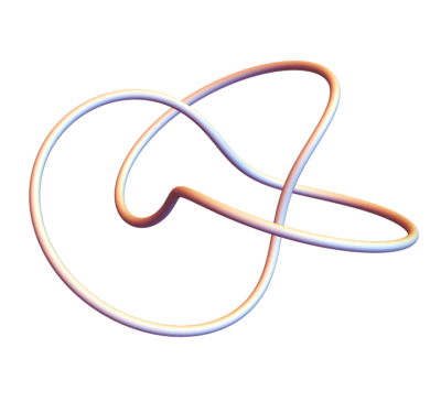
This is in fact a torus knot because the curve stays on the surface of a torus (doughnut) [1]. We can get a trefoil knot, for example, by setting p = 2 and q = 3.

We’ll use Mathematica to compute the total curvature of this knot and other examples. First the parameterization:

    x[t_, p_, q_] := Cos[p t] (Cos[q t] + 2)
    y[t_, p_, q_] := Sin[p t] (Cos[q t] + 2) 
    z[t_, p_, q_] := -Sin[q t]

We can plot torus knots as follows.

    k[t_, p_, q_] := { 
        x[t, p, q], 
        y[t, p, q], 
        z[t, p, q]
    }
    Graphics3D[Tube[Table[k[i, p, q], {i, 0, 2 Pi, 0.01}], 
        0.08], Boxed -> False]

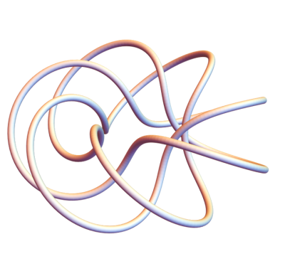
Here’s a more complicated knot with p = 3 and q = 7.

Before we can integrate the curvature with respect to arc length, we need an expression for an element of arc length as a function of the parameter t.

    ds[t_, p_, q_] :=  Sqrt[ 
        D[x[t, p, q], t]^2 + 
        D[y[t, p, q], t]^2 + 
        D[z[t, p, q], t]^2
    ]

Now we can compute the total curvature.

    total[p_, q_] := NIntegrate[
        ArcCurvature[k[t, p, q], t] ds[t, p, q], 
        {t, 0, 2 Pi}
    ]

We can use this to find that the total curvature of the (2,3) torus knot, the trefoil, is 17.8224, whereas 4π is 12.5664. So the Fary-Milnor theorem holds.

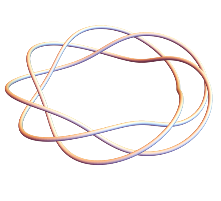
Let’s do one more example, this time a (1,4) knot.

You can see that this is not actually knot. This doesn’t contradict what we said above because 1 divides 4. When p or q equal 1, we get an unknot.

When we compute its total curvature we get 24.2737, more than 4π. The Fary-Milnor theorem doesn’t say that total curvature in excess of 4π is a sufficient condition for a loop to be knotted; it says it’s necessary. Total curvature less than 4π proves that something isn’t a knot, but curvature greater than 4π doesn’t prove anything.

More on curvature and knots

• Curvature and automatic differentiation
• Squircles and curvature
• Globe knots

[1] If you change out the 2s in the parameterization with a larger number, it’s easier to see from the graphs that the curves are on a torus. For example, if we plot the (3,7) knot again, replacing 2’s in the definition of x(t) and y(t) with 5’s, we can kinda see a torus inside the knot.