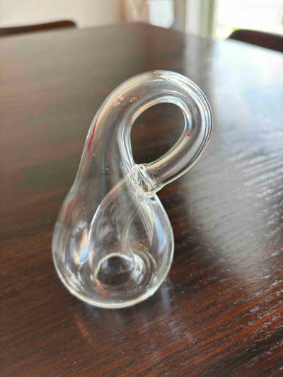
One of my daughters gave me a Klein bottle for Christmas.
Imagine starting with a cylinder and joining the two ends together. This makes a torus (doughnut). But if you twist the ends before joining them, much like you twist the ends of a rectangular strip to make a Möbius strip, you get a Klein bottle. This isn’t possible to do in 3D without making the cylinder pass through itself, so you’re supposed to imagine that the part where the bottle intersects itself isn’t there.
But is a Klein bottle real? My Christmas present is a real physical object, so it’s real in that sense. Is a Klein bottle real as a mathematical object? Can it be defined without any appeal to imagining things that aren’t true? Yes it can.
Formal definition
Start with a unit square, the set of points (x, y) with 0 ≤ x, y ≤ 1. If you identify the top and bottom of the square, the points with y coordinate equal to 0 or 1, you get a cylinder. You can imagine curling the square in 3D and taping the top and bottom together.
Similarly, if you start with the unit square and identify the vertical sides together with a twist, you get a Möbius strip. You won’t be able to physically do this with a square, but you could with a rectangle. Or you could imagine the square to be made out of rubber, and you stretch it before you twist it and join the edges together.
If you start with the unit square and do both things described above—join the top and bottom as-is and join the sides with a twist—you get a Klein bottle. You can’t quite physically do both at the same time in 3D; you’d have to cut a little hole in the square to let part of the square pass through, as in the glass bottle at the top of the post.
Although you can’t construct a physical Klein bottle without a bit of cheating, there’s nothing wrong with the mathematical definition. There are some details that have been left out, but there’s nothing illegal about the construction.
More formality
To fill in the missing details, we have to say just what we mean by identifying points. When we identify the top edge and bottom edge of the square to make a cylinder, we mean that we imagine that for every x, (x, 0) and (x, 1) are the same point. Similarly, when we identify the sides with a twist, we imagine that for all y, (0, y) and (1, 1 − y) are the same point.
But this is unsatisfying. What does all this imagining mean? How is this any better than imagining that the hole in the glass bottle isn’t there? We can define what it means to “identify” or “glue” edges together in a way that’s perfectly rigorous.
We can say that as a set of points, the Klein bottle is
K = [0, 1) × [0, 1),
removing the top and right edge. But what makes this set of points a Klein bottle is the topology we put on it, the way we define which points are close together.
We define an ε neighborhood of a point (x, 0) to be the union of two half disks, the intersection with K of an open disk of radius ε centered at (x, 0) and the intersection with K of an open disk centered at (x, 1). This is a way to make rigorous the idea of gluing (x, 0) and (x, 1) together.
Along the same lines, we define an ε neighborhood of a point (0, y) to be the intersection with K of an open disk of radius ε centered at (0, y) and an open disk of radius ε centered at (1, 1 − y).
The discussion with coordinates is more complicated than the talk about imagining this and that, but it’s more rigorous. You can’t have simplicity and rigor at the same time, so you alternate back and forth. You think in terms of the simple visualization, but when you’re concerned that you may be saying something untrue, you go down to the detail of coordinates and prove things carefully.
Topology can seem all hand-wavy because that’s how topologist communicate. They speak in terms of twisting this and glueing that. But they have in the back of their mind that all these manipulations can be justified. The formalism may be left implicit, even in a scholarly publication, when it’s assumed that the reader could fill in the details. But when things are more subtle, the formalism is written out.
Escaping 3D
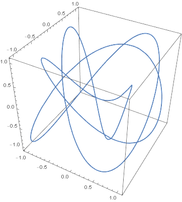
In the construction above, we define the Klein bottle as a set of points in the 2D plane with a new topology. That works, but there’s another approach. I said above that you can’t join the edges to make a Klein bottle in three dimensions. I added this disclaimer because you can join the edges without cheating if you work in higher dimensions.
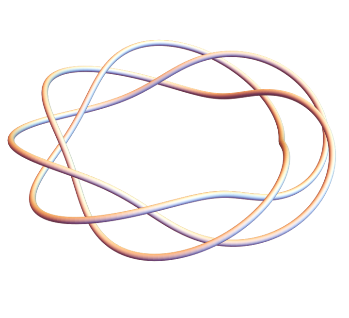
If you’d like a parameterization of the Klein bottle, say because you want to calculate something, you can do that, but you’ll need to work in four dimensions. There’s more room to move around in higher dimensions, letting you do things you can’t do in three dimensions.