Curvature is conceptually simple but usually difficult to calculate. For a level set curve f(x, y) = c, such as in the previous couple posts, the equation for curvature is

Even when f has a fairly simple expression, the expression for κ can be complicated.
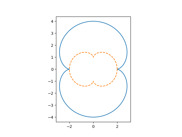
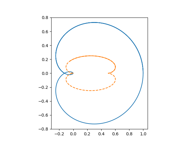
If we define
![]()
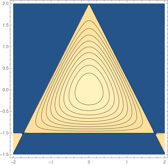
then the level set of f(x, y) = c is an equilateral triangle when c = −4. The level sets are smoothed triangles for −4 < c < 0.
The curvature of these level sets at any point is given by

Simplification
But there is one instance in which curvature is easy to calculate. For the graph of a function g(x) = y, the curvature is approximately the absolute value of the second derivative of g, provided the first derivative is small.
![]()
At a local maximum or local minimum of g(x) the approximation is exact because the first derivative is zero.
Max and min curvature of smoothed triangles
This means that in the example above, we can calculate the maximum and minimum curvature of the level sets. The maximum curvature occurs in the corners and the minimum occurs in the middle of the sides. By symmetry there are three maxima and three minima, but we can take the ones corresponding to x = 0 for convenience. There we find the curvature is simply
![]()
When x = 0, we have
![]()
and so the maximum and minimum curvature are the two roots of the cubic equation for y that lie in the interval [−1, 2]. (There’s another root greater than 2.)
For example, when c = −3, the roots are 0.8794, 1.3473, and 2.5321. The first root corresponds to the minimum curvature, the second to the maximum, and the third is outside our region of interest. It follows that the minimum curvature is 0.7237 and the maximum is 14.0838.
When c = −1 the minimum and maximum curvature are 2.80747 and 9.91622 respectively,
Since c = −4 corresponds to the triangle, the minimum curvature is 0 and the maximum is infinite. As c increases, the minimum and maximum curvature come together because the level set is becoming more round.