The Lorenz system is a canonical example of chaos. Small changes in initial conditions eventually lead to huge changes in the solutions.
And yet discussions of the Lorenz system don’t simply show this. Instead, they show trajectories of the system, which make beautiful images, but do not demonstrate the effect of small changes to initial conditions. Or they demonstrate it in two or three dimensions where it’s harder to see.
If you’ve seen the Lorenz system before, this is probably the image that comes to mind.
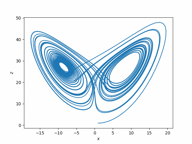
This plots (x(t), z(t)) for the solutions to the system of differential equations
x‘= σ(y − x)
y‘ = x(ρ − z) − y
z‘ = xy − βz
where σ = 10, ρ = 28, β = 8/3. You could use other values of these parameters, but these were the values originally used by Edward Lorenz in 1963.
The following plots, while not nearly as attractive, are more informative regarding sensitive dependence on initial conditions.
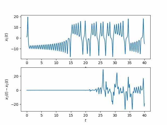
In this plot, x1 is the x-component of the solution to the Lorenz system with initial condition
(1, 1, 1)
and x2 the x-component corresponding to initial condition
(1, 1, 1.00001).
The top plot is x1 and the bottom plot is x1 − x2.
Notice first how erratic the x component is. That might not be apparent from looking at plots such as the plot of (x, z) above.
Next, notice that for two solutions that start off slightly different in the z component, the solutions are nearly identical at first: the difference between the two solutions is zero as far as the eye can tell. But soon the difference between the two solutions has about the same magnitude as the solutions themselves.
Below is the Python code used to make the two plots.
    from scipy import linspace
    from scipy.integrate import solve_ivp
    import matplotlib.pyplot as plt

    def lorenz(t, xyz):
        x, y, z = xyz
        s, r, b = 10, 28, 8/3. # parameters Lorentz used
        return [s*(y-x), x*(r-z) - y, x*y - b*z]

    a, b = 0, 40
    t = linspace(a, b, 4000)

    sol1 = solve_ivp(lorenz, [a, b], [1,1,1], t_eval=t)
    sol2 = solve_ivp(lorenz, [a, b], [1,1,1.00001], t_eval=t)

    plt.plot(sol1.y[0], sol1.y[2])
    plt.xlabel("$x$")
    plt.ylabel("$z$")
    plt.savefig("lorenz_xz.png")
    plt.close()

    plt.subplot(211)
    plt.plot(sol1.t, sol1.y[0])
    plt.xlabel("$t$")
    plt.ylabel("$x_1(t)$")
    plt.subplot(212)
    plt.plot(sol1.t, sol1.y[0] - sol2.y[0])
    plt.ylabel("$x_1(t) - x_2(t)$")
    plt.xlabel("$t$")
    plt.savefig("lorenz_x.png")
One important thing to note about the Lorenz system is that it was not contrived to show chaos. Meteorologist and mathematician Edward Lorenz was lead to the system of differential equations that bears his name in the course of his work modeling weather. Lorenz understandably assumed that small changes in initial conditions would lead to small changes in the solutions until numerical solutions convinced him otherwise. Chaos was a shocking discovery, not his goal.
Those plots are in Lorenz’s paper but as you point out they are seldom seen now (but should be).
Little appreciated fact: these equations were derived by Lorenz and Saltzman using what we now call compression techniques
So how accurate are these plots? If the system is extremely sensitive to a small change in the position at time 0, we would expect it to be sensitive to a small change at time, say, 1, which could be caused by floating point error. Of course, the floating point error is much smaller than 0.00001, but I would expect the error to get larger with each step. Or does SciPy have some clever way to avoid these errors?
It would be interesting to plot as well the absolute error | x_1 – x_2 | – not as attractive as your plot, but would illustrate the long-term behaviour of the error.