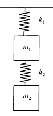
Imagine a spring with stiffness k1 attached to a ceiling and a mass m1 handing from the spring.
There’s a second spring attached to the first mass with stiffness k2 and a mass m2 handing from that.
The motion of the system is described by the pair of differential equations
![]()
If the second spring were infinitely stiff, the two masses would be joined with a rigid rod, and so the system would act like a single mass m1 + m2 hanging from the first spring. This motion would be described by the single differential equation
![]()
So it’s not surprising that as k2 gets stiffer, the solution to the two-mass system converges to the solution to the system with a single combined mass. This is proven in [1].
However, what is missing from [1] is any visualization of how the solution to the two-mass system converges to that of the combined-mass system.
The plot below shows solutions for k2 equal to 10, 100, and 1000, and finally the system to the combined-mass system, labeled k2 = ∞. I used k1 = 1, m1 = 3, and m2 = 5.
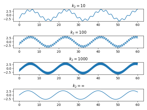
The coupled-mass system has a high-frequency component due to the oscillation of the second mass relative to the first one.
The authors in [1] show that the amplitude of the high-frequency component decays as k2 goes to infinity, though this is not apparent from the plots above. This is due to a limitation of the numerical method used to produce the plots.
Analytical solution
The numerical solution above raises two questions. First, how fast should the amplitude of high frequency component decay. Second, why did the numerical method apparently get the frequency of this component correct but the amplitude wrong?
The second question is more difficult and will have to wait for another post. The first question, however, we can settle fairly quickly.
The authors in [1] make the simplifying assumption that the two masses are equal to 1. They then define show that
![]()
where the d‘s are constants that depend on initial conditions but not on the spring stiffnesses. and

α4, the frequency of the low frequency component, approaches a finite limit as k2 → ∞,
α2, the frequency of the high frequency component, is approximately √(2k2) for large k2.
The amplitude of the high frequency component should be inversely proportional to its frequency.
More differential equation posts
[1] K. E. Clark and S. Hill. The Effects of a Stiffening Spring. The College Mathematics Journal , Nov., 1999, Vol. 30, No. 5 (Nov., 1999), pp. 379-382
I’m reminded of Gibbs’ phenomenon. Does the high frequency component disappear simply by virtue of its amplitude approaching zero at infinite stiffness, or is it something more complicated somehow also involving its wavelength approaching zero?
The amplitude of the high frequency component should be inversely proportional to the frequency, according to the analytical solution. It’s interesting that the numerical solution captures the increasing frequency but does not capture the decreasing amplitude.
I imagine an energy-preserving numerical method would do better. Something to explore in a future post.
What are the initial conditions used? If you implement individual displacement conditions on the masses it may account for the seemingly constant amplitude of the harmonic. Such IC would of course only be relevant for a finite k2.
I think the second equation has a small typo — it’s x1 instead of x2?
m2*x2” = -k2*(x2-x1)
Yeah, the amplitude of that high frequency component looks strongly stable over three orders of magnitude. Hope you get a chance to investigate further.
Gotta love coupled systems.
In the mid-1990s I worked on the Stationary Neutron Radiography System (SNRS) at what was then McClellan Air Force Base in Sacramento, which is now called the McClellan Nuclear Radiation Center run by UC Davis ( https://mnrc.ucdavis.edu/).
The overall system was awesome: We punched holes in the side of a Triga nuclear research reactor to produce carefully collimated neutron beams of very high intensity to search for hidden corrosion within aluminum, titanium and magnesium honeycomb aircraft wings and skin components by detecting and measuring neutron scattering caused by the hydrogen in the hydrides of corrosion. These large aircraft components were moved through the beam by an enormous 7 DOF gantry-style robot.
As the lead software engineer, my primary responsibilities were the neutron radiography imaging system, including real-time video processing, and the operator interfaces for both the imaging and robotics. When we started doing our initial all-up system performance and certification runs, the giant robot started displaying motion instabilities that were causing hydraulic safety valves to lift, fittings to fail, motion system circuit breakers to open, electrical motors to burn out, and axes to hit their hard end-stops causing the entire structure to distort. I was tasked to help with the investigation (well, everyone was).
While the mechanical engineers were working on repairing and beefing up the mechanical structure and hydraulic actuators, and the electrical engineers worked on repairing the motion control systems and making them more robust, I worked on characterizing the system behavior with the goal of modifying the control algorithms to avoid overload and instability, starting with a simple rod and spring model, followed by a carefully designed system stimulation routine to gather performance information without breaking the robot (again).
My model was crude in the extreme, hardly acknowledging the actual robot design, which frustrated the mechanical engineers. I mainly wanted a framework on which to hang experimental evidence, not to derive or predict system behavior from first principles.
The data gathering started with locking all robot axes (literally bolting them together) then moving the outermost axis and monitoring system behavior via accelerometers on each axis. This proceeded to unlocking the other axes one at a time and repeating the motion program, adding the new axis. Each additional axis multiplied the testing time, as all axis combinations were permuted, meaning I was pulling long overnight shifts until the data collection was completed.
My investigatory motion control program excited some awesome flex in the robot, just as intended, but which freaked-out everyone else, despite not causing any system damage or causing any safety systems to engage. This was on a multi-ton system specified to provide millimeter-level position repeatability summed across all axes, and I had it waving like a blowy-man at a gas station (comparatively speaking).
The first thing everyone wanted to do was to make the robot stiffer, which I pointed out would also make it heavier, and risk worsening the effects of any instabilities. But I had to prove it, or at least provide strong evidence.
The analysis was simple in the extreme: Feed the data through FFTs and look for resonances. All I did was provide control algorithm modifications that would avoid exciting the resonant nodes and limit the flex revealed in the data, and added a gentle pre-scan motion routine to determine where the nodes would be based on the robot gantry payload (which ranged from pounds to tons, awkwardly distributed). The resulting data was used to conservatively limit axis velocity, acceleration and jerk.
The initial software update successfully completed a scan without problems, but it was very slow as the limits were extremely conservative. A few iterations refined the behavior to yield a net system performance improvement, as accelerations and velocities could be increased where there were no instabilities or resonances.
The mechanical engineers were frustrated I didn’t provide them with anything more than my experimental data and some frequency plots: I never bothered to derive the set of coupled motion differential equations, mainly because I didn’t want to parameterize the entire payload space for the robot and then develop part positioning routines to minimize problems. Just provide the robot with a few basic rules, then let it figure out how best to safely move.
I referred everyone to what I called “the Principle of Maximal Ignorance” to illustrate the problem was complex enough to be inherently indeterminate, especially as we couldn’t predict the future uses of the system nor how its behavior would change with age. So I didn’t bother trying, instead choosing to rely on a handful of system fundamentals and hardware limits, without an elaborate model. The accelerometers provided the “Minimal Knowledge” needed to dynamically detect out-of-bounds behavior well before it caused problems.
The accelerometers were augmented with hydraulic pressures and electrical amperages both to sanity-check the accelerometers and to ensure interactive and automated control inputs had their expected effects.
The maxim is true: Software engineers are lazy! I really didn’t want to develop a system physics model I doubted would work or even be useful if it worked perfectly.
Our physicists and mechanical engineers couldn’t let go of the problem, and a year later an internal report was circulated containing a detailed mechanical model that made useful predictions, but which didn’t lead to any software changes. Well, couldn’t lead to software changes: By the time the report was completed, the robot had evolved considerably.
What’s fun is that I recently used a similar approach to optimize the motion of my 3D printer (which exhibited some Z-axis resonances). Which, from my perspective, is just another gantry robot, and a simple one at that. I was positively giddy while gluing $2 accelerometers to the base frame and to each axis, reveling in acquiring, analyzing and presenting the data in a JupyterLab notebook. So much faster, easier, cheaper, more accurate and just better overall than 25 years ago!
@BobC very interesting anecdote!