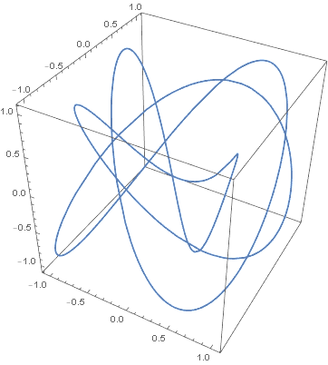
Several months ago I wrote a blog post about Lissajous curves and knots that included the image below.
Here’s an improved version of the same knot.
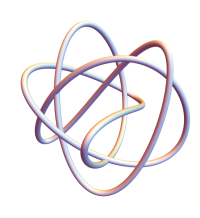
The original image was like tying the knot in thread. The new image is like tying it in rope, which makes it easier to see. The key was to use Mathematica’s Tube function to thicken the curve and to see the crossings. I also removed the bounding box in the image.
This was the original code:
    x[t_] := Cos[3 t]
    y[t_] := Cos[4 t + Sqrt[2]]
    z[t_] := Cos[5 t + Sqrt[3]]

    ParametricPlot3D[{x[t], y[t], z[t]}, {t, 0, 2 Pi}]
The new code keeps the definitions of x, y, and z but creates a plot using Tube.
    Graphics3D[
        Tube[
             Table[{x[i], y[i], z[i]}, {i, 0, 2 Pi, 0.01}],
             0.05
        ],
        Boxed -> False
    ]
I went back and changed out the plots in my post Total curvature of a knot with plots similar to the one above.
The lowest crossing in the ‘tube’ diagram looks like an intersection, in which case we don’t have a standard knot. In the original ‘line’ diagram, that area of the graph seems more complex.