The previous post looked at a cellular automaton introduced by Edward Fredkin. It has only two states: a cell is on or off. At each step, each cell is set to the sum of the states of the neighboring cells mod 2. So a cell is on if it had an odd number neighbors turned on, and is turned off if it had an even number of neighbors turned on.
You can look at cellular automata with more states, often represented as colors. If the number of states per cell is prime, then the extension of Fredkin’s automaton to multiple states also reproduces its initial pattern. Instead of taking the sum of the neighboring states mod 2, more generally you take the sum of the neighboring states mod p.
This theorem is due to Terry Winograd, cited in the same source as in the previous post.
Here’s an example with 11 states. The purple background represents 0. As before, I start with an ‘E’ pattern, but I make it multi-colored.
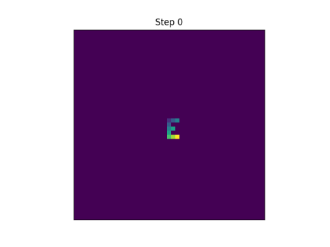
Before turn on the automaton, we need to clarify what we mean by “neighborhood.” In this example, I mean cells to the north, south, east, and west. You could include the diagonals, but that would be different example, though still self-reproducing.
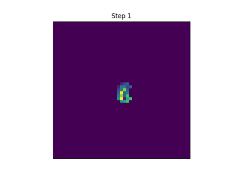
After the first step, the pattern blurs.
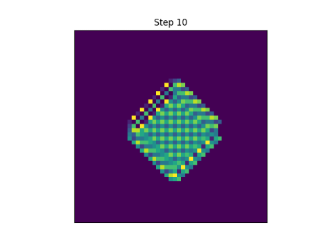
After 10 steps the original pattern is nowhere to be seen.
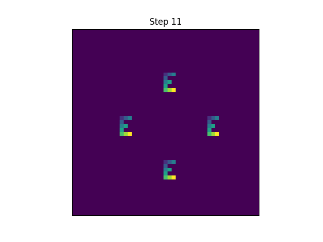
And then suddenly on the next step the pattern reappears.
I don’t know whether there are theorems on how long it takes the pattern to reappear, or how the time depends on the initial pattern, but in my experiments, the a pattern reappears after 4 steps with 2 states, 9 steps with 3 states, 5 steps with 5 states, 7 steps with 7 states, and 11 steps with 11 states.
Here’s an animation of the 11-color version, going through 22 steps.

I find it interesting, in this post and the last one, how the second-to-last state looks so ordered. In a way it makes sense (it has to collapse back to being mostly zeroes), but as you say, it’s hard to even find a hint of the original in there. But run it for one time step, and there it is.
The problem is additive, right? The state of a cell after N steps is the sum (mod p) of its N-step states where only one cell of the original pattern was actually active. So then the question is how a single 1 propagates through the grid. After p steps the (±p, 0) and (0, ±p) points will certainly contain 1, and my feeling is that all other points will be 0, since the initial 1 will have arrived there some multinomial coefficient number of times divisible by p. So if your pattern is smaller in size than p pixels, then in p steps it would be replicated 4 times. If it’s larger, then the 4 copies would overlap, and I guess p^2 would be the next possible clean time.
I believe Ivan is correct. More specifically, starting from a single 1 the state of a cell after n steps is the number of n-step walks from the original 1 to that cell. If n = p, all such walks will occur in multiples of p except for those consisting of p steps in the same direction (this can be shown either by looking at multinomial coefficients or by a symmetry argument). For multiples of p steps, we’re essentially dealing with the same cellular automaton but moving by p spaces instead of 1, so any pattern smaller than p pixels is replicated every p steps, and we can repeat this argument recursively to deal with powers of p.
For more fun, if the modulus is a product of distinct primes, we can decompose, for example, Z_{pq} into the product of Z_p and Z_q. For example, for this pattern with a height of 5 pixels, if the modulus is 6, we should see something like a replicating pattern after 72 steps, with 4 distinct copies of the original pattern in the cardinal directions and some other copies, some of them overlapping, in between.