Multicolor reproducing cellular automata

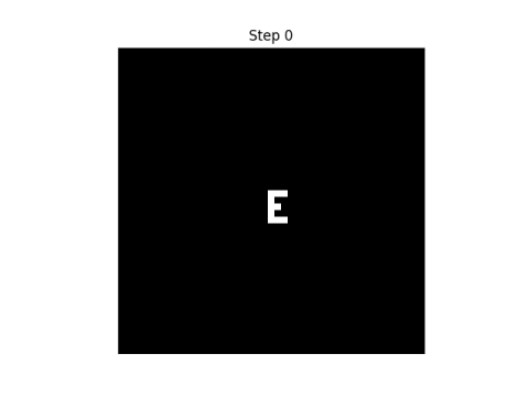
The previous post looked at a cellular automaton introduced by Edward Fredkin. It has only two states: a cell is on or off. At each step, each cell is set to the sum of the states of the neighboring cells mod 2. So a cell is on if it had an odd number neighbors turned on, and is turned off if it had an even number of neighbors turned on.

You can look at cellular automata with more states, often represented as colors. If the number of states per cell is prime, then the extension of Fredkin’s automaton to multiple states also reproduces its initial pattern. Instead of taking the sum of the neighboring states mod 2, more generally you take the sum of the neighboring states mod p.

This theorem is due to Terry Winograd, cited in the same source as in the previous post.

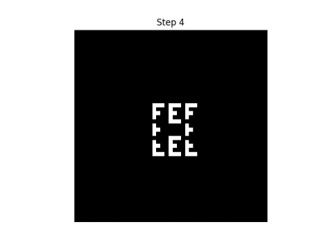
Here’s an example with 11 states. The purple background represents 0. As before, I start with an ‘E’ pattern, but I make it multi-colored.

Initial state

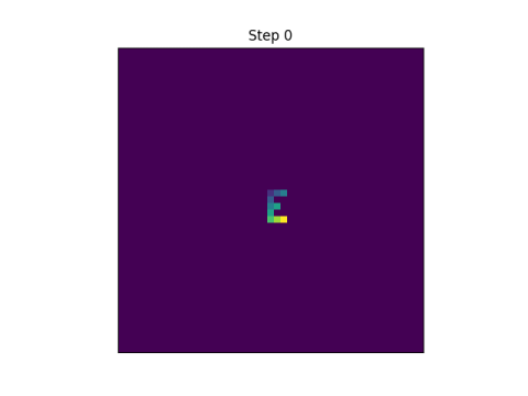
Before turn on the automaton, we need to clarify what we mean by “neighborhood.” In this example, I mean cells to the north, south, east, and west. You could include the diagonals, but that would be different example, though still self-reproducing.

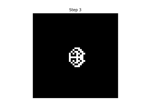
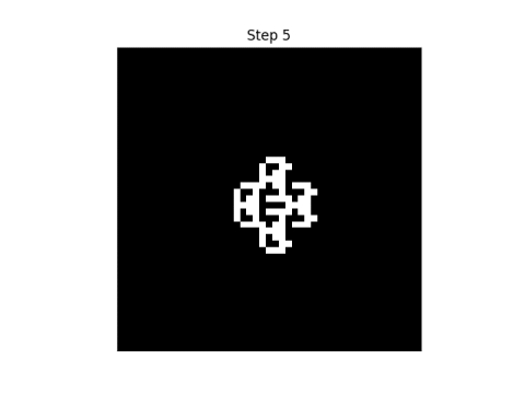
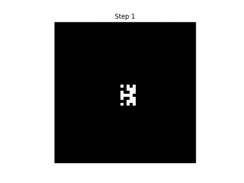
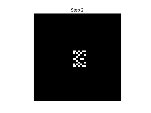
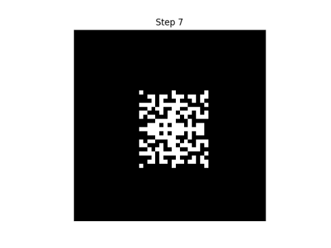
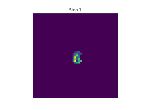
After the first step, the pattern blurs.

step 1

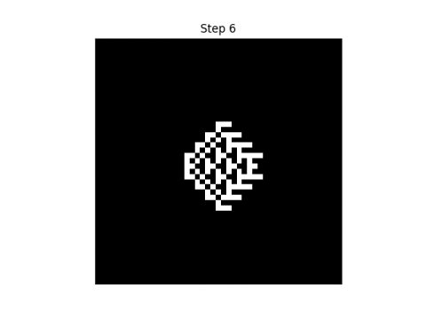
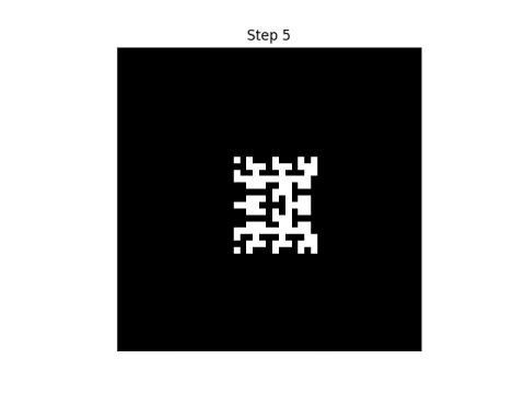
After 10 steps the original pattern is nowhere to be seen.

step 10

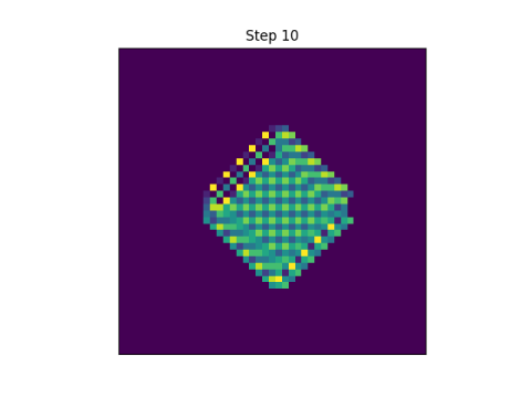
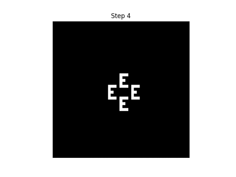
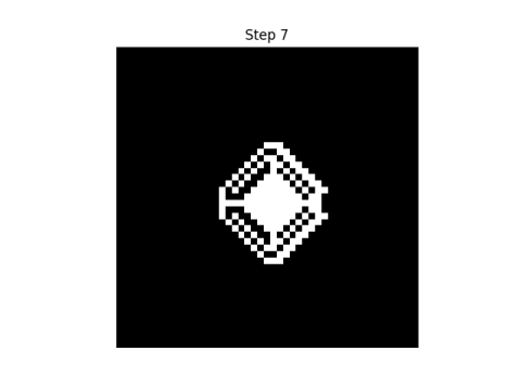
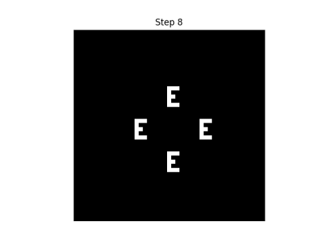
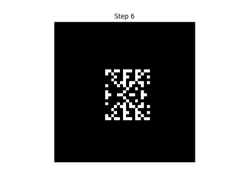
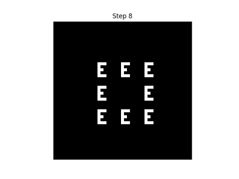
And then suddenly on the next step the pattern reappears.

step 11

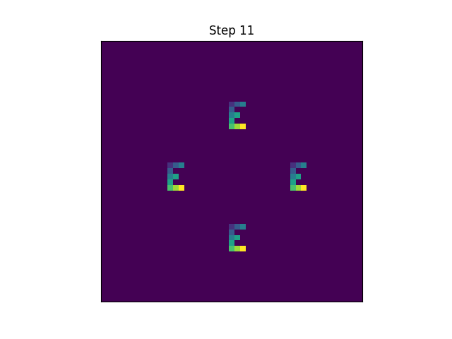
I don’t know whether there are theorems on how long it takes the pattern to reappear, or how the time depends on the initial pattern, but in my experiments, the a pattern reappears after 4 steps with 2 states, 9 steps with 3 states, 5 steps with 5 states, 7 steps with 7 states, and 11 steps with 11 states.

Here’s an animation of the 11-color version, going through 22 steps.

Animated gif of CA

Self-reproducing cellular automata

Edward Fredkin is best known these days for the Fredkin gate, a universal reversible circuit.

I recently found out that Fredkin was one of the pioneers in cellular automata. His student Edwin Banks describes a cellular automaton introduced by Fredkin [1].

Edward Fredkin of MIT has described the following interesting cellular space. If the states are 0 and 1 and if the result state is obtained by taking the sum of the neighbors, modulo 2, then every initial configuration will reproduce copies of itself about the initial configuration.

In other words, start with some bit pattern in an infinite checkerboard of bits. Then at each step, replace each bit by the parity of the sum of the neighboring bits. Eventually you’ll see copies of that original pattern.

There’s some ambiguity regarding what “neighbors” means. Banks’ dissertation considers the neighbors of a bit to be the bits to the north, south, east, and west, and this implies that Banks has these neighbors in mind when he describes Fredkin’s automaton. Other sources say Fredkin also considered diagonally adjacent bits as part of the neighborhood, i.e. northwest, northeast, southwest, and southeast.

Banks goes on to say

Terry Winograd (1970) generalized this result showing that any neighborhood, not just the four nearest neighbors, and any number of dimensions still yields the same results.

I take it by “the four nearest neighbors” the neighbors to the north, south, east, and west. I’m not sure what the “any neighborhood” means in Winograd’s theorem; I imagine there must be some implied restriction.

In any case, I’ll show by example that both definitions of “neighborhood” discussed above lead to reproducing the original pattern, though they do not reproduce it in the same way.

I’ll start with an ‘E’ in the middle of a grid. The black squares represent 0s and the white squares represent 1s.

initial state

Here are the first eight steps in evolving this pattern, using the rule that “neighbor” only includes north, south, east, and west neighbors.

If we consider each point to have eight neighbors, i.e. we include diagonals, here’s what the first eight steps look like.

Update: Here’s an animated version of the first automaton

and the second

See the next post for a generalization using more than two states per cell, using colors rather than black and white cells. If the number of colors is prime, and you take the sum of the neighboring states mod p rather than mod 2, you get analogous results.

[1] Edwin R. Banks, Information Processing and Transmission in Cellular Automata. MIT dissertation. January 1971.

Powers of 3 in binary

I was thumbing through A New Kind of Science [1] and one of the examples that jumped out at me was looking at the bits in the binary representation of the powers of 3. I wanted to reproduce the image myself and here’s the result.

bits of powers of 3 plotted

Here a white square represents a 1 and a blue square a 0. There’s a white border on the right edge because all powers of 3 are odd, i.e. end in 1 when written in binary.

As with many of the images in Wolfram’s book, it’s somewhere between regular and chaotic.

I produced the image at the command line with the following Python code.

    from numpy import log2

    N = 60
    k = int(log2(3)*N)+1

    for i in range(N):
        s = format(3**i, str(k)+'b')
        s = s.replace('1', chr(0x2588))
        s = s.replace('0', ' ')
        print(s)

The code writes powers of three as binary strings of length k where k is calculated so the last number in the sequence will fit. It then replaces 1s with a solid block character and replaces 0s with a blank space. My terminal has a blue background and a white foreground, so 1s show up as white squares and 0s as blue.

The characters in my terminal are twice as high as they are wide, so I changed the aspect ratio after taking the screen shot so that the blocks come out more square.

Update: Other bases

What if we look at bases other than 3?

Here’s the revised code to let you specify any base b.

    from numpy import log2

    def out(s):
        s = s.replace('1', chr(0x2588))
        s = s.replace('0', ' ')
        print(s)    

    b = 5
    N = 50
    k = int(log2(b)*N)+1

    for i in range(N):
        s = format(b**i, str(k)+'b')
        out(s)

Here’s what powers of 5 look like:

bits of powers of 5 plotted

And here’s what powers of 7 look like:

bits of powers of 7 plotted

What if our base isn’t prime? It doesn’t make an obvious difference if the base is odd, but if it’s even we get a skewed image. Here’s the plot for p = 6.

bits of powers of 6 plotted

This is just the plot for powers of 3 with the nth row shifted left by n positions.

Related posts

[1] I’ve looked through the book before for fun, but this time I’m looking through it with a practical project in mind. I never thought that would happen.

Cellular automata with random initial conditions

The previous post looked at a particular cellular automaton, the so-called Rule 90. When started with a single pixel turned on, it draws a Sierpinski triangle. With random starting pixels, it draws a semi-random pattern that retains features like the Sierpinski triangle.

There are only 256 possible elementary cellular automata, so it’s practical to plot them all. I won’t list all the images here—you can find them all here—but I will give a few examples to show the variety of patterns they produce. As in the previous post, we imagine our grid rolled up into a cylinder, i.e. we’ll wrap around if necessary to find pixels diagonally up to the left and right.

rule 8 with random initial conditions
rule 18 with random initial conditions
rule 29 with random initial conditions
rule 30 with random initial conditions
rule 108 with random initial conditions
rule 129 with random initial conditions

As we discussed in the previous post, the number of a rule comes from what value it assigns to each of eight possible cellular states, turned into a binary number. So it’s plausible that binary numbers with more 1’s correspond to more black pixels. This is roughly true, though the graph below shows that the situation is more complex than that.

automata pixel density as a function of 1 bits in rule