Suppose you do N trials of something that can succeed or fail. After your experiment you want to present a point estimate and a confidence interval. Or if you’re a Bayesian, you want to present a posterior mean and a credible interval. The numerical results hardly differ, though the two interpretations differ.
If you got half successes, you will report a confidence interval centered around 0.5. The more unbalanced your results were, the smaller your confidence interval will be. That is, the confidence interval will be smallest if you had no successes and widest if you had half successes.
What can we say about how the width of your confidence varies as a function of your point estimate p? That question is the subject of this post [1].
Frequentist confidence interval width
We’ll start with an example, where N = 1,000,000. We let our number of observed successes n vary from 0 to 500,000 and plot the width of a 95% confidence interval as a function of n on a log-log plot. (By symmetry we only need to look to up to N/2. If you have more than half successes, reverse your definitions of success and failure.)
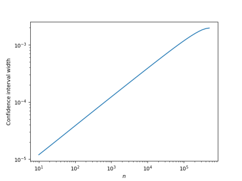
The result is almost a perfectly straight line, with the exception of a tiny curve at the end. This says the log of the confidence interval is a linear function of the log of n, or in other words, the dependence of confidence interval width on n follows a power law.
Bayesian credible interval width
The plot above measures frequentist confidence intervals, using Wilson score with continuity correction. We can repeat our experiment, putting on our Bayesian hat, and compute credible intervals using a Jeffreys prior, that is, a beta(0.5, 0.5) prior.
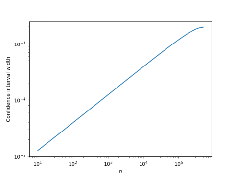
The results are indistinguishable. The confidence interval widths differ after the sixth decimal place.
In this example, there’s very little quantitative difference between a frequentist confidence interval and a Bayesian credible interval. The difference is primarily one of interpretation. The Bayesian interpretation makes sense and the frequentist interpretation doesn’t [2].
Power law
If the logs of two things are related linearly [3], then the things themselves are related by a power law. So if confidence/credible interval width varies as a power law with the point estimate p, what is that power law?
The plots above suggest that to a good approximation, if we let w be the credible interval length,
log w = m log p + b
for some slope m and intercept b.
We can estimate the slope by choosing p = 10−1 and p = 10−5. This gives us m = 0.4925 and b = −5.6116. There are theoretical reasons to expect that m should be 0.5, so we’ll round 0.4925 up to 0.5 both for convenience and for theory.
So
log w = 0.5 log p − 5.6116.
and so
w = 0.00366 √p
Let’s see how well this works by comparing it to the exact interval length. (I’m using Jeffreys’ credible interval, not that it matters.)
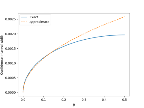
The power law approximation works well when the estimated proportion p is small, say less than 0.2. For larger p the normal approximation works well.
We could have guessed that the confidence interval width was proportional to √p(1−p) based on the normal approximation/central limit theorem. But the normal approximation is not uniformly good over the range of all ps.
Related posts
- Bounding the probability of something that hasn’t happened yet
- Predictive probability for large populations
- Computing normal probabilities with a basic calculator
[1] Standard notation would put a little hat on top of the p but HTML doesn’t make this possible without inserting images into text. I hope you don’t mind if I take my hat off.
[2] This quip is a little snarky, but it’s true. When I would ask graduate students to describe what a confidence interval is, they would basically give me the definition of a credible interval. Most people who calculate frequentist confidence intervals think they’re calculating Bayesian credible intervals, though they don’t realize it. The definition of confidence interval is unnatural and convoluted. But confidence intervals work better in practice than in theory because they approximate credible intervals.
L. J. Savage once said
“The only use I know for a confidence interval is to have confidence in it.”
In other words, the value of a confidence interval is that you can often get away with interpreting it as a credible interval.
[3] Unfortunately the word “linear” is used in two inconsistent ways. Technically we should say “affine” when describing a function y = mx + b, and I wish we would. But that word isn’t commonly known. People call this relation linear because the graph is a line. Which makes sense, but it’s inconsistent with the use of “linear” as in “linear algebra.”
Hi John,
At the end of the day, as a Stats useful, I don’t really want to have to keep these 2 interpretation differences in my head all the time. Since what’s wanted is credible interval, but instead confidence interval is calculated, are there ways the Stats experts can improve the situation? For example, alculate credible interval or an accurate approximation of it, within the frequentist framework? Note: I don’t have a preference to either frameworks, I think we need to make it easier to use Stats is the viewpoint coming from.