Richard Feynman said that almost everything becomes interesting if you look into it deeply enough. Looking up numbers in a table is certainly not interesting, but it becomes more interesting when you dig into how well you can fill in the gaps.
If you want to know the value of a tabulated function between values of x given in the table, you have to use interpolation. Linear interpolation is often adequate, but you could get more accurate results using higher-order interpolation.
Suppose you have a function f(x) tabulated at x = 3.00, 3.01, 3.02, …, 3.99, 4.00 and you want to approximate the value of the function at π. You could approximate f(π) using the values of f(3.14) and f(3.15) with linear interpolation, but you could also take advantage of more points in the table. For example, you could use cubic interpolation to calculate f(π) using f(3.13), f(3.14), f(3.15), and f(3.16). Or you could use 29th degree interpolation with the values of f at 3.00, 3.01, 3.02, …, 3.29.
The Lagrange interpolation theorem lets you compute an upper bound on your interpolation error. However, the theorem assumes the values at each of the tabulated points are exact. And for ordinary use, you can assume the tabulated values are exact. The biggest source of error is typically the size of the gap between tabulated x values, not the precision of the tabulated values. Tables were designed so this is true [1].
The bound on order n interpolation error has the form
c hn + 1 + λ δ
where h is the spacing between interpolation points and δ is the error in the tabulated values. The value of c depends on the derivatives of the function you’re interpolating [2]. The value of λ is at least 1 since λδ is the “interpolation” error at the tabulated points.
The accuracy of an interpolated value cannot be better than δ in general, and so you pick the value of n that makes c hn + 1 less than δ. Any higher value of n is not helpful. And in fact higher values of n are harmful since λ grows exponentially as a function of n [3].
See the next post for mathematical details regarding the λs.
Examples
Let’s look at a specific example. Here’s a piece of a table for natural logarithms from A&S.
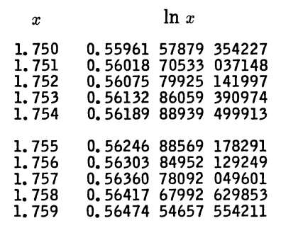
Here h = 10−3, and so linear interpolation would give you an error on the order of h² = 10−6. You’re never going to get error less than 10−15 since that’s the error in the tabulated values, so 4th order interpolation gives you about as much precision as you’re going to get. Carefully bounding the error would require using the values of c and λ above that are specific to this context. In fact, the interpolation error is on the order of 10−8 using 5th order interpolation, and that’s the best you can do.
I’ll briefly mention a couple more examples from A&S. The book includes a table of sine values, tabulated to 23 decimal places, in increments of h = 0.001 radians. A rough estimate would suggest 7th order interpolation is as high as you should go, and in fact the book indicates that 7th order interpolation will give you 9 figures of accuracy,
Another table from A&S gives values of the Bessel function J0 in with 15 digit values in increments of h = 0.1. It says that 11th order interpolation will give you four decimal places of precision. In this case, fairly high-order interpolation is useful and even necessary. A large number of decimal places are needed in the tabulated values relative to the output precision because the spacing between points is so wide.
Related posts
[1] I say were because of course people rarely look up function values in tables anymore. Tables and interpolation are still widely used, just not directly by people; computers do the lookup and interpolation on their behalf.
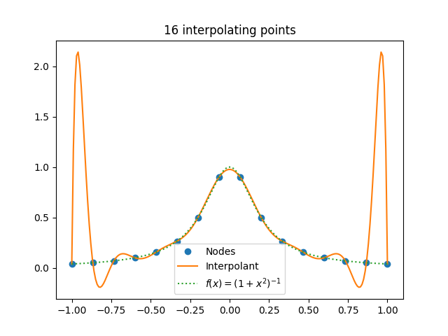
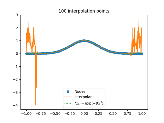
[2] For functions like sine, the value of c doesn’t grow with n, and in fact decreases slowly as n increases. But for other functions, c can grow with n, which can cause problems like Runge phenomena.
[2] The constant λ grows exponentially with n for evenly spaced interpolation points, and values in a table are evenly spaced. The constant λ grows only logarithmically for Chebyshev spacing, but this isn’t practical for a general purpose table.