If a single server is being pushed to the limit, adding a second server can drastically reduce wait times. This is true whether the server is a human serving food or a computer serving web pages. I first wrote about this here and I give more details here.
What if you add an extra server but you also add more customers? The second server still reduces the wait time, though clearly not by as much as if the work load didn’t increase.
If you increase the number of servers in proportion to the traffic, wait times will go down. In theory, wait times will approach zero as the traffic and number of servers go off to infinity together. So under ideal assumptions, you could lower wait times by scaling your number of customers and your number of servers. Alternatively, you could scale your number of servers but not as fast as your number of customers, and keep wait times constant while reducing payroll.
In theory, the ideal scale is as large as possible. Economies of scale are real, but so are dis-economies of scale. Eventually the latter overtakes the former. But that’s a matter for another post. For this post we’re only looking at an idealized model.
Examples
As before we assume the time between customer arrivals and the time required to serve each customer is random. (Technically, a M/M/s model.)
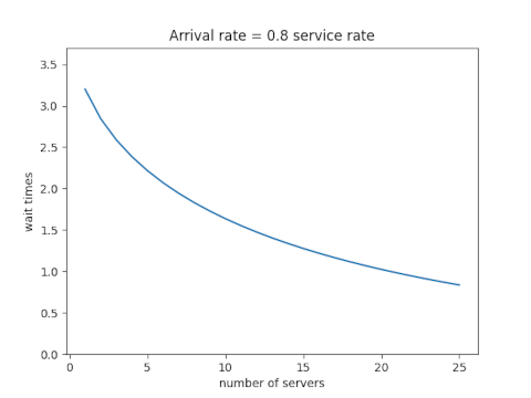
Assume first that the ratio of the rate at which customers arrive to the rate at which they can be served is 0.8. Here’s what happens when we increase the traffic and the number of servers proportionally.
Next assume that the ratio of the arrival and service rates is 0.9. Scaling the traffic and servers proportionally reduces the number of customers in line, but the wait time declines more slowly than it did when each server wasn’t so close to capacity.
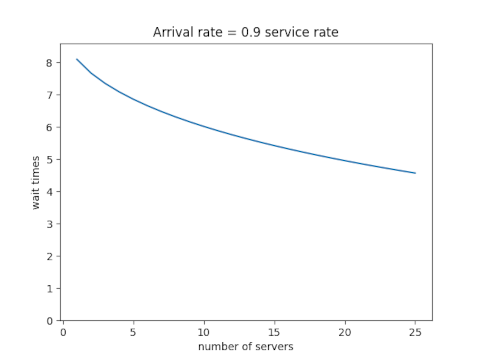
Each new server helps, but each helps less than the one before. You hit diminishing return immediately.
Equations
Let ρ be the ratio of the total arrival rate to the rate at which a single server can take care of a customer and let s be the number of servers. In the examples above, ρ was 0.8s and 0.9s. The equations below don’t assume any particular relation between ρ and s except that ρ/s must be less than 1. (If ρ/s were greater than 1, the system would not approach an equilibrium; lines would grow without bound over time.)
Define p0 as follows. (NB: that’s a Roman p, not a Greek ρ. They’re visually similar, but it’s conventional notation in queueing theory.)

Then the expected wait time is

By the way, we’ve assumed the time between arrivals and the time to serve a customer are both exponentially distributed. What if they’re not? That is the subject of my next post.
Label on the 2nd graph is incorrect (should be 0.9).
Thanks.