Brian Christian and Tom Griffiths have just published a new book, Algorithms at Work.
You can hear me talking about queues in Episode 2.
Brian Christian and Tom Griffiths have just published a new book, Algorithms at Work.
You can hear me talking about queues in Episode 2.
The previous post presented an approximation for the steady-state wait time in queue with a general probability distribution for inter-arrival times and for service times, i.e. a G/G/s queue where s is the number of servers. This post will give an upper bound for the wait time.
Let σ²A be the variance on the inter-arrival time and let σ²S be the variance on the service time. Then for a single server (G/G/1) queue we have
![]()
where as before λ is the mean number of arrivals per unit time and ρ is the ratio of lambda to the mean number of customers served. The inequality above is an equality for the Markov (M/M/1) model.
Now consider the case of s servers. The upper bound is very similar for the G/G/s case
![]()
and reduces to the G/G/1 case when s = 1.
Source: Donald Gross and Carl Harris. Fundamentals of Queueing Theory. 3rd edition.
Textbook presentations of queueing theory start by assuming that the time between customer arrivals and the time to serve a customer are both exponentially distributed.
Maybe these assumptions are realistic enough, but maybe not. For example, maybe there’s a cutoff on service time. If someone takes too long, you tell them there’s no more you can do and send them on their merry way. Or maybe the tails on times between arrivals are longer than those of an exponential distribution.
The default model makes other simplifying assumptions than just the arrival and service distributions. It also makes other simplifying assumptions. For example, it assumes no balking: customers are infinitely patient, willing to wait as long as necessary without giving up. Obviously this isn’t realistic in general, and yet it might be adequate when wait times are short enough, depending on the application. We will remove the exponential probability distribution assumption but keep the other assumptions.
Assuming exponential gaps between arrivals and exponential service times has a big advantage: it leads to closed-form expressions for wait times and other statistics. This model is known as a M/M/s model where the two Ms stand for “Markov” and the s stands for the number of servers. If you assume a general probability distribution on arrival gaps and service times, this is known as a G/G/s model, G for “general.”
The M/M/s model isn’t just a nice tractable model. It’s also the basis of an approximation for more general models.
Let A be a random variable modeling the time between arrivals and let S be a random variable modeling service times.
The coefficient of variation of a random variable X is its standard deviation divided by its mean. Let cA and cS be the coefficients of variation for A and S respectively. Then the expected wait time for the G/G/s model is approximately proportional to the expected wait time for the corresponding M/M/s model, and the proportionality constant is given in terms of the coefficients of variation [1].
![]()
Note that the coefficient of variation for an exponential random variable is 1 and so the approximation is exact for exponential distributions.
How good is the approximation? You could do a simulation to check.
But if you have to do a simulation, what good is the approximation? Well, for one thing, it could help you test and debug your simulation. You might first calculate outputs for the M/M/s model, then the G/G/s approximation, and see whether your simulation results are close to these numbers. If they are, that’s a good sign.
You might use the approximation above for pencil-and-paper calculations to get a ballpark idea of what your value of s needs to be before you refine it based on simulation results. (If you refine it at all. Maybe the departure of your queueing system from M/M/s is less important than other modeling considerations.)
[1] See Probability, Statistics, and Queueing Theory by Arnold O. Allen.
If a single server is being pushed to the limit, adding a second server can drastically reduce wait times. This is true whether the server is a human serving food or a computer serving web pages. I first wrote about this here and I give more details here.
What if you add an extra server but you also add more customers? The second server still reduces the wait time, though clearly not by as much as if the work load didn’t increase.
If you increase the number of servers in proportion to the traffic, wait times will go down. In theory, wait times will approach zero as the traffic and number of servers go off to infinity together. So under ideal assumptions, you could lower wait times by scaling your number of customers and your number of servers. Alternatively, you could scale your number of servers but not as fast as your number of customers, and keep wait times constant while reducing payroll.
In theory, the ideal scale is as large as possible. Economies of scale are real, but so are dis-economies of scale. Eventually the latter overtakes the former. But that’s a matter for another post. For this post we’re only looking at an idealized model.
As before we assume the time between customer arrivals and the time required to serve each customer is random. (Technically, a M/M/s model.)
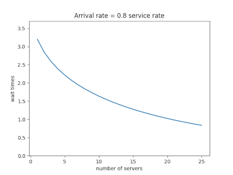
Assume first that the ratio of the rate at which customers arrive to the rate at which they can be served is 0.8. Here’s what happens when we increase the traffic and the number of servers proportionally.
Next assume that the ratio of the arrival and service rates is 0.9. Scaling the traffic and servers proportionally reduces the number of customers in line, but the wait time declines more slowly than it did when each server wasn’t so close to capacity.
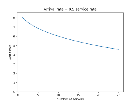
Each new server helps, but each helps less than the one before. You hit diminishing return immediately.
Let ρ be the ratio of the total arrival rate to the rate at which a single server can take care of a customer and let s be the number of servers. In the examples above, ρ was 0.8s and 0.9s. The equations below don’t assume any particular relation between ρ and s except that ρ/s must be less than 1. (If ρ/s were greater than 1, the system would not approach an equilibrium; lines would grow without bound over time.)
Define p0 as follows. (NB: that’s a Roman p, not a Greek ρ. They’re visually similar, but it’s conventional notation in queueing theory.)

Then the expected wait time is

By the way, we’ve assumed the time between arrivals and the time to serve a customer are both exponentially distributed. What if they’re not? That is the subject of my next post.
A blog post about queueing theory that I wrote back in 2008 continues to be popular. The post shows that when a system is close to capacity, adding another server dramatically reduces the wait time. In that example, going from one teller to two tellers doesn’t make service twice as fast but 93 times as fast.
That post starts out at a very high level and then goes into some details. This post goes into much more detail.
For a quick introduction to queueing theory, see this page.
In Kendall’s notation, we’re talking about M/M/1 and M/M/2 queues. The first letter denotes the assumed distribution on times between customer arrivals, the second denotes the distribution on service times, and the number at the end gives the number of servers.
The simplest and most common models in queueing theory are M/M models. The M‘s stand for “Markov” but they really mean exponential. (Sorry. I didn’t invent the notation.) The time between arrivals is exponentially distributed, which means the arrival is a Poisson process. The time it takes to serve each customer is also exponentially distributed.
Let λ be the number of who arrive per unit time, and let μ be the number of customers served per unit time, on average. For the system to approach a steady state we must have λ/μ < 1. Otherwise the number of customers in the queue grows over time without bound. In the example I mentioned above, λ = 5.8 customers per hour, and μ = 6 customers per hour. Customers are coming in nearly as fast as they can be served, and so a long line develops.
For a M/M/1 queue, the expected wait time, once the system reaches steady state, is
![]()
and the expected number of customers waiting at any time is
![]()
The equations for M/M/k systems in general are significantly more complicated, but they’re not bad when k = 2. For an M/M/2 system at steady state, the expected wait time is
![]()
and the expected number of customers waiting is
![]()
You may have noticed that for both M/M/1 and M/M/2 the expected number of customers waiting in line is λ times the expected wait time, i.e. L = λW. This is true in general and is known as Little’s law.

Queueing theory is the study of waiting in line. That may not sound very interesting, but the subject is full of surprises. For example, when a server is near capacity, adding a second server can cut backlog not just in half but by an order of magnitude or more. More on that here.
In this post, I’m not going to look at the content of queueing theory but just the name. When seeing the word queueing, many people assume it is misspelled and want to replace it with queuing. As I write this, my spell checker is recommending that change. But the large majority of people in the field call their subject queueing theory.
Queueing has five consecutive vowels. Are there any other English words with so many vowels in a row? To find out, I did an experiment like the classic examples from Kernighan and Pike demonstrating regular expressions by searching a dictionary for words with various patterns.
The first obstacle I ran into is that apparently Ubuntu doesn’t come with a dictionary file. However this post explains how to install one.
The second obstacle was that queueing wasn’t in the dictionary. I first searched the American English dictionary, and it didn’t include this particular word. But then I searched the British English dictionary and found it.
Now, to find all words with five consecutive vowels, I ran this:
egrep '[aeiou]{5}' british-english
and got back only one result: queueing. So at least in this dictionary of 101,825 words, the only word with five (or more) consecutive vowels is queueing.
Out of curiosity I checked how many words have at least four consecutive vowels. The command
grep -E "[aeiou]{4}" british-english | wc -l
returns 40, and the corresponding command with the file american-english returns 39. So both dictionaries contain 39 words with exactly four vowels in a row and no more. But are they the same 39 words? In fact they are. And one of the words is queuing, and so apparently that is an acceptable spelling in both American and British English. But as a technical term in mathematics, the accepted spelling is queueing.
Some of the 39 words are plurals or possessives of other words. For example, the list begins with Hawaiian, Hawaiian’s, and Hawaiians. (Unix sorts capital letters before lower case letters.) After removing plurals and possessives, we have 22 words with four consecutive vowels:
It’s interesting that three of the words are related to Hawaii: Kauai is an Hawaiian island and Kulauea is a Hawaiian volcano.
I’d never heard of Quaoar before. It’s a Kuiper belt object about half the size of Pluto.

There’s a branch of math that studies how people wait in line: queueing theory. It’s not just about people standing in line, but about any system with clients and servers.
An introduction to queueing theory, about what you’d learn in one or two lectures, is very valuable for understanding how the world around you works. But after a brief introduction, you quickly hit diminishing return on your effort, unless you want to specialize in the theory or you have a particular problem you’re interested in.
The simplest models in queueing theory have nice closed-form solutions. They’re designed to be easy to understand, not to be highly realistic in application. They make simplifying assumptions, and minor variations no longer have nice solutions. But they make very useful toy models.
One of the insights from basic queueing theory is that variability in arrival and service times matters a great deal. This is unlike revenue, for example, where you can estimate total revenue simply by multiplying the estimated number of customers by the estimated average revenue per customer.
A cashier who can handle a stream of customers on average could be in big trouble. If customers arrived at regular intervals and all required the same amount of time to serve, then if things are OK on average, they’re OK. But if there’s not much slack, and there’s the slightest bit of variability in arrival or service times, long lines will form.
I work through a specific example here. The example also shows that when a system is near capacity, adding a new server can make a huge improvement. In that example, going from one server to two doesn’t just cut the waiting time in half, but reduces it by a couple orders of magnitude.
As I mentioned at the beginning, queueing theory doesn’t just apply to shoppers and cashiers. It also applies to diverse situations such as cars entering a highway and page requests hitting a web server. See more on the latter here.
Joel Spolsky of Joel on Software fame mentions queueing theory in the latest StackOverflow podcast. He mentions a rule of thumb that wait times go up quickly as server utilization exceeds 80%. The same principle applies whether you’re talking about computer servers or human servers. I hadn’t heard of that rule of thumb, though I knew that you don’t want anywhere near 100% utilization. Here’s the graph that justifies Joel’s remark.
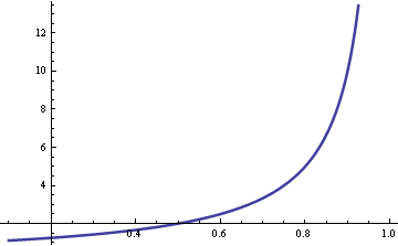
The vertical axis is wait time. The horizontal access is utilization.
Here are the details. Basic queuing theory assumes customer arrivals are Poisson distributed with rate λ. Service times are exponentially distributed with rate μ. The ratio λ/μ is called utilization ρ. If this ratio is greater than 1, that says customers are arriving faster than they can be served, and so the line will grow without bound. If the ratio is less than 1, the line will reach some steady state on average.
The average waiting time is W = 1/(μ-λ). Now assume the service time μ is fixed and the arrival rate λ = ρ μ. Then W = 1/μ(1-ρ) and so the wait time is proportional to 1/(1-ρ). As the utilization ρ approaches 1, the wait time goes to infinity. The graph above plots 1/(1-ρ). As Joel said, the curve does go up quickly when ρ exceeds 0.8.
Related post: What happens when you add a new teller?
Suppose a small bank has only one teller. Customers take an average of 10 minutes to serve and they arrive at the rate of 5.8 per hour. What will the expected waiting time be? What happens if you add another teller?
We assume customer arrivals and customer service times are random (details later). With only one teller, customers will have to wait nearly five hours on average before they are served. But if you add a second teller, the average waiting time is not just cut in half; it goes down to about 3 minutes. The waiting time is reduced by a factor of 93x.
Why was the wait so long with one teller? There’s not much slack in the system. Customers are arriving every 10.3 minutes on average and are taking 10 minutes to serve on average. If customer arrivals were exactly evenly spaced and each took exactly 10 minutes to serve, there would be no problem. Each customer would be served before the next arrived. No waiting.
The service and arrival times have to be very close to their average values to avoid a line, but that’s not likely. On average there will be a long line, 28 people. But with a second teller, it’s not likely that even two people will arrive before one of the tellers is free.
Here are the technical footnotes. This problem is a typical example from queuing theory. Customer arrivals are modeled as a Poisson process with λ = 5.8/hour. Customer service times are assumed to be exponential with mean 10 minutes. (The Poisson and exponential distribution assumptions are common in queuing theory. They simplify the calculations, but they’re also realistic for many situations.) The waiting times given above assume the model has approached its steady state. That is, the bank has been open long enough for the line to reach a sort of equilibrium.
Queuing theory is fun because it is often possible to come up with surprising but useful results with simple equations. For example, for a single server queue, the expected waiting time is λ/(μ(μ − λ)) where λ the arrival rate and μ is the service rate. In our example, λ = 5.8 per hour and μ = 6 per hour. Some applications require more complicated models that do not yield such simple results, but even then the simplest model may be a useful first approximation.
Update: More details and equations here. Non-technical overview of queueing theory here.