You might think that if zip codes are close, then the regions they represent are close. Or that if zip codes are consecutive, then their regions touch. Neither of these are true. I explore how far they are from being true in the next post.
But these statements could have been true [1]. It’s possible to lay a grid on a region and number the squares in the grid in such a way that consecutive numbers correspond to contiguous squares, and nearby numbers correspond to nearby squares. There are geocoding systems that accomplish this using Hilbert curves. For example, Google’s S2 system is based on Hilbert curves.
A Hilbert curve is a curve that winds through a square, coming arbitrarily close to every point in the square. A Hilbert curve is a fractal, defined as the limit of an iterative process. We aren’t concerned with the limit because we only want to carry out a finite number of steps in the construction. But the fact that the limit exists tells us that with enough steps we can get any resolution we want.
To illustrate Hilbert curves and how they could be used to label grids, we will use a Hilbert curve to tour a chessboard. We will number the squares of a chess board so that consecutive numbers correspond to neighboring squares.
Here’s Python code to produce our numbering.
    from hilbertcurve.hilbertcurve import HilbertCurve

    p = 3 # 2^3 squares on a side
    n = 2 # two dimensional cube, i.e. square

    hc = HilbertCurve(p, n)

    for row in range(2**p):
        for col in range(2**p):
            d = hc.distance_from_point([row, col])
            print(format(d,"2d"), " ", end="")
        print()
This produces the following output.
     0   1  14  15  16  19  20  21
     3   2  13  12  17  18  23  22
     4   7   8  11  30  29  24  25
     5   6   9  10  31  28  27  26
    58  57  54  53  32  35  36  37
    59  56  55  52  33  34  39  38
    60  61  50  51  46  45  40  41
    63  62  49  48  47  44  43  42
Here’s Python code to draw lines rather than print numbers.
    N = (2**p)**n
    points = hc.points_from_distances(range(N))

    for i in range(1, N):
        x0, y0 = points[i-1]
        x1, y1 = points[i]
        plt.plot([x0, x1], [y0, y1])
    plt.gca().set_aspect('equal')
    plt.show()
This produces the following image.
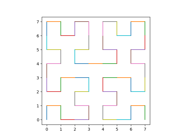
There’s a small problem. Following the square numberings above produces a Hilbert curve, and the plotting code produces and Hilbert curve, but they’re not the same Hilbert curve. The implicit axes created by our sequence of print statements doesn’t match the geometry in the plotting code. To get the curves to match we need to do a sort of change of coordinates. We can do this by changing the call to plt.plot to
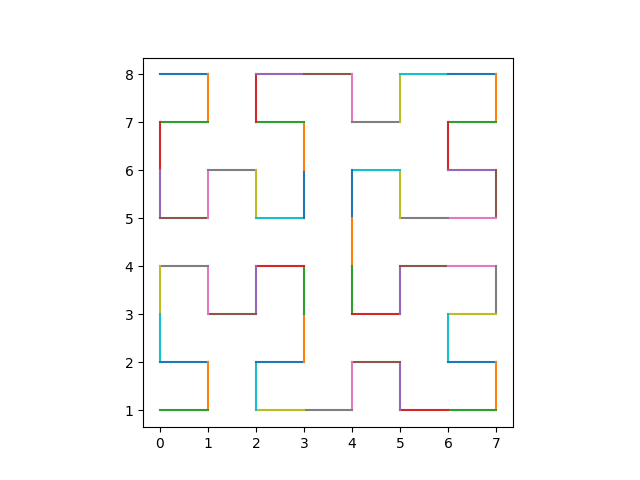
plt.plot([y0, y1], [8-x0, 8-x1])
This produces the following plot, matching the numbering above.
Related posts
[1] It could have been true in the sense that it was theoretically possible. It might not have been practically possible. Postal codes have different design constraints than geocodes.
Another astonishing property of the Hilbert curve, besides its maintaining “closeness” is that it really, truly crosses every point in the square, in the infinite limit, naturally. In other words, it’s a _bona fide_ map \(\mathbb{R}\to\mathbb{R}^2\) since the square has the same measure as the whole \(\mathbb{R}^2\) plane. It wasn’t historically the first space-filling curve, but the first smooth map (most jagged curve yields the most smooth map!!!). Even more interesting property is that this map doesn’t have an inverse, i.e. there is a set of points that it maps at least twice. Fascinating stuff!
Whence’s “from hilbertcurve.hilbertcurve import HilbertCurve”? The only ways I know of constructing the curve is via the L-system, or a trivially similar clone-rotate-connect, probably the most well-known construction. I’m wondering what’s inside this package.
I rather enjoy the power of a hilbert curve … the above python hilbertcurve library lives at `https://pypi.org/project/hilbertcurve/` source at https://github.com/galtay/hilbertcurve
I have written some golang code which uses a hilbert curve to determine the path to traverse an image where the first pixel is given some audio frequency and each subsequent pixel an incrementally higher audio freq … it then aggregates all of those audio oscillators into a single audio signal … this is the hard way of doing the inverse fourier transform of the image … beauty is this audio can then be given to other code which is the above algorithm in reverse which can listen to the audio and pop out an image … much joy then that output image finally matched the source input image … currently making that audio more human listening friendly to hopefully allow the blind to see by listening to whatever they point their cell phone camera at … ditto for the deaf who might be able to suss out say an incoming phone call by viewing the visual representation of the the other person talking