A couple years ago I wrote about how NASA was interested in regions bounded by curves of the form
![]()
For example, here’s a plot for A = 2, B = 1, α = 2.5 and β = 6.
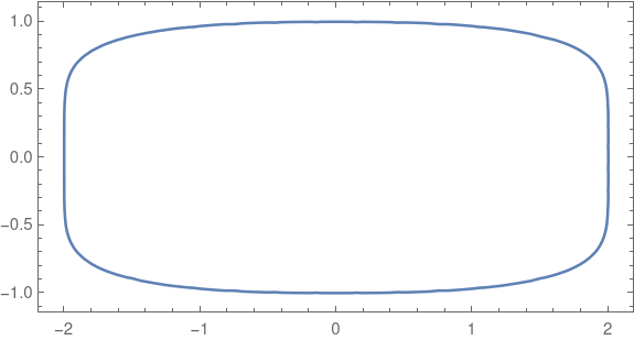
That post mentioned a technical report from NASA that explains why these shapes are important in application, say for beams and bulkheads, and gives an algorithm for finding conformal maps of the unit disk to these shapes. These shapes are also used in graphic design, such as squircle buttons on iPhones.
Note that these shapes are not rounded rectangles in the sense of a rectangles modified only at the corners. No segment of the sides is perfectly flat. The curvature smoothly decreases as you move away from the corners rather than abruptly jumping to 0 as it does in a rectangle rounded only at the corners. Maybe you could call these shapes continuously rounded rectangles.
Conformal maps
Conformal maps are important because they can map simple regions to more complicated regions in way that locally preserves angles. NASA might want to solve a partial differential equation on a shape such as the one above, say to calculate the stress in a cross section of a beam, and use conformal mapping to transfer the equation to a disk where the calculations are easier.
Coefficients
The NASA report includes a Fortran program that computes the coefficients for a power series representation of the conformal map. All the even coefficients are zero by reasons of symmetry.
Coefficients are reported to four decimal places. The closer the image is to a circle, i.e. the closer α and β are to 2 and the closer A is to B, the fewer non-zero coefficients the transformation has. You could think of the number of non-zero coefficients as a measure how hard the transformation has to work to transform the disk into the desired region.
There are interesting patterns in the coefficients that I would not have noticed if I had not had to type the coefficients into a script for the example below. Maybe some day I’ll look more into that.
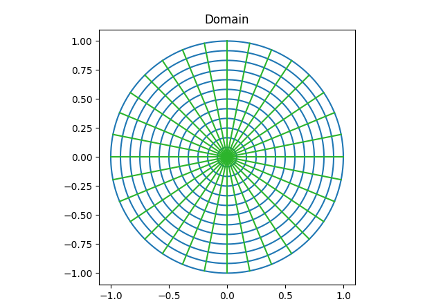
Conformal map example
The following example uses A = 2, B = 1, and α = β = 5.
We start with the following disk with polar coordinate lines drawn.
And here is the image of the disk under the conformal map giving by the coefficients in the NASA report.
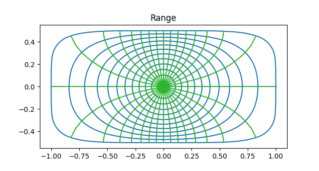
Note that the inner most circles from the domain are mapped into near circles, but as you move outward the circles are distorted more, approaching the shape of the boundary of the range.This is because in the limit, analytic functions map disks to disks. So a tiny circle around the origin will always map to an approximate circle, regardless the target region.
Note also that although the circles and lines of the domain are warped in the range, they warp in such a way that they still intersect at right angles. This is the essence of a conformal map.
Inverse map
The NASA report only gives a way to compute the transformation from the disk to the target region. Typically you need to be able to move both ways, disk to target and target to disk. However, since the transformation is given by a power series, computing the inverse transformation is a problem that has been solved in general. This post gives an explanation and an example.