In the previous post I looked at graphs created from representing geographic regions with nodes and connecting nodes with edges if the corresponding regions share a border.
It’s an interesting exercise to recover the geographic regions from the network. For example, take a look at the graph for the continental United States.
It’s easy to identify Alaska in the graph. The node on the left represents Maine because Maine is the only state to border exactly one other state. From there you can bootstrap your way to identifying the rest of the states.
Math class
This could make a fun classroom exercise in a math class. Students will naturally come up with the idea of the degree of a node, the number of edges that meet that node, because that’s a handy way to solve the puzzle: the only possibilities for a node of degree n are states that border n other states.
This also illustrates that networks preserve topology, not geometry. That is, the connectivity information is retained, but the shape is dramatically different.
Geography class
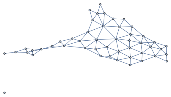
Someone asked me on Twitter to make a corresponding graph for Brazil. Mathematica, or at least my version of Mathematica, doesn’t have data on Brazilian states, so I made an adjacency graph using GraphViz.
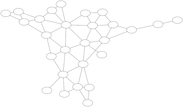
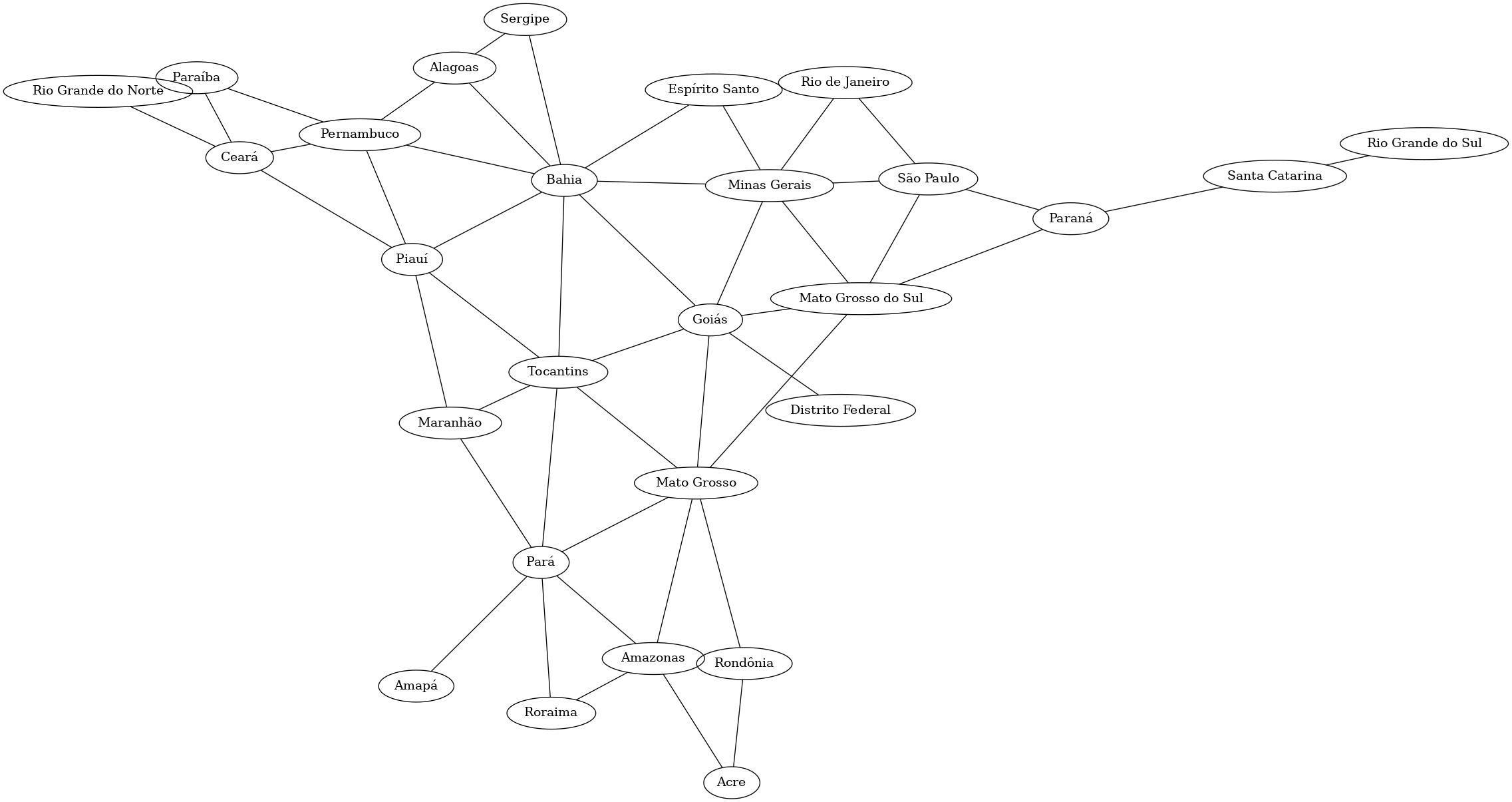
Labeling the blank nodes is much easier for Brazil than for the US because Brazil has about half as many states, and the topology of the graph gives you more to work with. Three nodes connect to only one other node, for example.
Here the exercise doesn’t involve as much logic, but the geography is less familiar, unless of course you’re more familiar with Brazil than the US. Labeling the graph will require staring at a map of Brazil and you might accidentally learn a little about Brazil.
GraphViz
The labeled version of the graph above is available here. And here are the GraphViz source files that make the labeled and unlabeled versions.
The layout of a GraphViz file is very simple. The file looks like this:
    graph G {

        layout=sfdp

        AC [label="Acre"]
        AL [label="Alagoas"]
        ...
        AC -- AM
        AC -- RO
        ...
    }
There are three parts: a layout, node labels, and connections.
GraphViz has several layout engines, and the sfdp one matched what I was looking for in this case. Other layout options lead to overlapping edges that were confusing.
The node names AC, AL, etc. do not appear in the output. They’re just variable names for your convenience. The text inside the label is what appears in the final output. I’ll give an example in the next post in which it’s very convenient for the variables to be different from the labels. The order of the labels doesn’t matter, only which variables are associated with which labels.
Finally, the lines with variables separated by dashes are the connection data. Here we’re telling GraphViz to connect node AC to nodes AM and RO. The order of these lines doesn’t matter.