In rectangular coordinates, constant values of x are vertical lines and constant values of y are horizontal lines. In polar coordinates, constant values of r are circles and constant values of θ are lines from the origin.
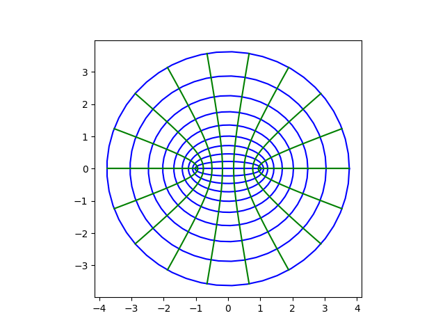
In elliptic coordinates, the position of a point is specified by two numbers, μ and ν. Constant values of μ are ellipses and constant values of ν are hyperbolas. (Elliptic coordinates could just as easily have been called hyperbolic coordinates, but in applications we’re usually more interested in the ellipses and so the conventional name makes sense.)
As with rectangular and polar coordinates, elliptic coordinates are orthogonal, i.e. holding each coordinate constant separately gives two curves that are perpendicular where they intersect.
Here’s a plot, with curves of constant μ in blue and curves of constant ν in green.
The correspondence between rectangular and elliptic coordinates is given below.
x = a cosh μ cos ν
y = a sinh μ sin ν
The value of a can be chosen for convenience. More on that below.
Notice that elliptic coordinates area approximately polar coordinates when μ is large. This is because cosh(μ) approaches sinh(μ) as μ increases. For small values of μ elliptic coordinates are very different from polar coordinates.
The purpose of various coordinate systems is to adapt your coordinates to the structure of your problem. If you’re working with something that’s radially symmetric, polar coordinates are natural. And if you’re working with an ellipse, say you’re computing the electric field of an ellipse with uniform charge, then elliptic coordinates are natural. Ellipses can be described by one number, the value of μ.
Separation of variables
However, the real reason for specialized coordinate systems is solving partial differential equations. (Differential equations provided the motivation for a great deal of mathematics; this is practically an open secret.)
When you first see differential equations, the first, and possibly only, technique for solving PDEs you see is separation of variables. If you have PDE for a function of two variables u(x, y), you first assume u is the product of a function of x alone and a function of y alone:
u(x, y) = X(x) Y(y).
Then you stick this expression into your PDE and get independent ODEs for X and Y. Then sums of the solutions (i.e. Fourier series) solve your PDE.
Now, here’s the kicker. We could do the same thing in elliptic coordinates, starting from the assumption
u(μ, ν) = M(μ) N(ν)
and stick this into our PDE written in elliptic coordinates. The form of a PDE changes when you change coordinates. For example, see this post on the Laplacian in various coordinate systems. When you leave rectangular coordinates, the Laplacian is no longer simply the sum of the second partials with respect to each variable. However, separation of variables still works for Laplace’s equation using elliptic coordinates.
Separable coordinate systems get their name from the fact that the separation of variables trick works in that coordinate system. Not for all possible PDEs, but for common PDEs like Laplace’s equation. Elliptic coordinates are separable.
If you’re solving Laplace’s equation on an ellipse, say with a constant boundary condition, the form of the solution is going to be complicated in rectangular coordinates, but simpler in elliptic coordinates.
Confocal elliptic coordinates
The coordinate ellipses, curves with μ constant, are ellipses with foci at ±a; you can choose a so that a particular ellipse you’re interested has a particular μ value, such as 1. Since all these ellipses have the same foci, we say they’re confocal. But confocal elliptic coordinates are something slightly different.
Elliptic coordinates and confocal elliptic coordinates share the same coordinate curves, but they label them differently. Confocal elliptic coordinates (σ, τ) are related to (ordinary) elliptic coordinates via
σ = cosh μ
τ = cos ν
Laplace’s equation is still separable under this alternate coordinate system, but it looks different; the expression for the Laplacian changes because we’ve changed coordinates.