Irving Burr came up with a set of twelve probability distributions known as Burr I, Burr II, …, Burr XII. The last of these is by far the best known, and so the Burr XII distribution is often referred to simply as the Burr distribution [1]. See the next post for the rest of the Burr distributions.
Cumulative density functions (CDFs) of probability distributions don’t always have a closed form, but it’s convenient when they do. And the CDF of the Burr XII distribution has a particularly nice closed form:
![]()
You can also add a scale parameter the usual way.
The flexibility of the Burr distribution isn’t apparent from looking at the CDF. It’s obviously a two-parameter family of distributions, but not all two-parameter families are equally flexible. Flexibility is a fuzzy concept, and there are different notions of flexibility for different applications. But one way of measuring flexibility is the range of (skewness, kurtosis) values the distribution family can have.
The diagram below [2] shows that the Burr distribution can take on a wide variety of skewness and kurtosis combinations, and that for a given value of skewness, the Burr distribution has the largest kurtosis of common probability distribution families. (Note that the skewness axis increases from top to bottom.)
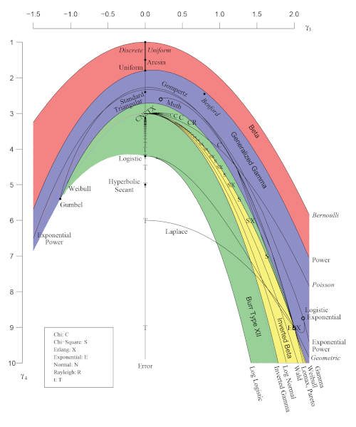
The green area at the bottom of the rainbow belongs to the Burr distribution. The yellow area is a subset of the green area.
[1] In economics the Burr Type XII distribution is also known as the Singh-Maddala distribution.
[2] Vargo, Pasupathy, and Leemis. Moment-Ratio Diagrams for Univariate Distributions. Journal of Quality Technology. Vol. 42, No. 3, July 2010. The article contains a grayscale version of the image, and the color version is available via supplementary material online.
I don’t understand a lot of it, but that is a great diagram!