How well does a spline fit a function?

Suppose you’re going to fit a spline s to a function f by interpolating f at a number of points. What can you know a priori about how well s will approximate f?

This question was thoroughly resolved five decades ago [1], but the result is a bit complicated, so we’ll incrementally work our way up to the final result.

What kind of spline

First of all we’ll need to be specific about what we mean by a spline. We’re going to look at cubic splines over a finite interval [a, b]. A cubic spline approximation to f over [a, b] is constructed by splitting the interval into N subintervals and fitting a cubic polynomial to f over each subinterval. The piecewise polynomials much match the value of f at the ends of the subintervals, and the values over contiguous intervals much match their first and second derivatives.

We’re not going to specify the endpoint conditions of the spline. The spline described above is not unique; it has two degrees of freedom which are typically specified by boundary conditions, but the theorem we’re building up to doesn’t require us to say anything about boundary conditions. In particular, we do not require our spline to be a natural cubic spline.

How to measure fit

How should we measure how well our spline s fits our function f? Obviously we’d like have a bound on

|s(x) – f(x)|

at each point. We’d also like to have a bound on the difference in derivatives at each point. Since our spline has two continuous derivatives, we’re interested in the first and second derivatives. In symbols, we’d like to bound

|s^(r)(x) – f^(r)(x)|

for r = 0, 1, or 2.

Smoothness of f

We have to say something about the smoothness of the function we’re interpolating. Since we’re appoximating f by a function with two continuous derivatives, it only makes sense to consider functions f with at least two derivatives. Typically f will be smoother than s, so we will also look at the case of f having three or four continuous derivatives. We will measure the smoothness of f by the maximum value of its derivatives over the interval [a, b]. That is, by

|f ^(m)|_∞

where m = 2, 3, or 4.

Mesh size

Obviously the accuracy of our approximation will depend on the number of interpolation points N+1. We will not require the interpolation points to be evenly spaced, and so we will quantify the fineness of our mesh as the length h of the longest subinterval of [a, b].

Shape of our theorem

We now have the elements we need to state our theorem. The left side will be

|s^(r)(x) – f^(r)(x)|

and the right side will be some expression involving r, n, h, and the values of

|f ^(m)|_∞

for varying values of m.

We can make the bound on the left side tighter by taking into account which subinterval j = 0, 1, 2, … N-1 our x belongs to. In general, spline interpolation is more accurate toward the middle of [a, b] than toward the edges. Interestingly, our theorem will only depend on j and not on the width of the jth interval.

The theorem

And now for the theorem we’ve been working our way up to:

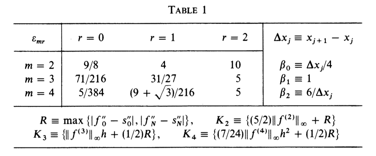
|s^(r)(x) – f^(r)(x)| ≤ ε_mr |f^(m)|_∞h^m–r+ K_mβ_r(2^1-j + 2^1-N+j) h.

The statement of the theorem is complicated because the author is carefully quantifying the error. You could make the theorem much simpler by just making a big-O statement. Instead, the author gives numerical values of each of the constants.

The theorem is even a little more complicated than it looks at first because the constants K_m depend on |f^(m)|_∞h. The values of the constants in the theorem are given in the table below. You can click on the image to get a larger image that is easier to read.