Rolling correlation

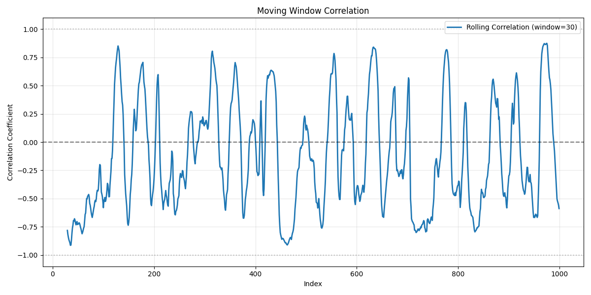
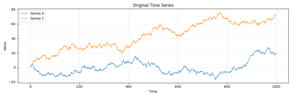
Suppose you have data on the closing prices of two stocks over 1,000 days and you want to look at the correlation between the two asset prices over time in rolling 30 day windows.

It seems that the rolling correlation is periodic. peaking about every 50 days.

But this is an artifact of the rolling window, not a feature of the data. I created the two simulated stock time series by creating random walks. The price of the stock each day is the price the previous day plus a sample from a normal random variable with mean zero and variance 1.

import numpy as np
from scipy.stats import norm

n = 1000
x = np.cumsum(norm.rvs(size=n))
y = np.cumsum(norm.rvs(size=n))    

If you use a wider window, say 60 days, you’ll still see a periodic pattern in the rolling correlation, though with lower frequency.

Related posts

True growth rate accounting for inflation

In an inflationary economy, the purchasing power of your currency continually deteriorates. If you have an investment that grows slower than your purchasing power shrinks, you’re actually losing value over time. The true rate of growth is the rate of change in the purchasing power of your investiment.

If the inflation rate is r and the rate of growth from your investment is i, then intuitively the true rate of growth is

g = ir.

But is it? That depends on whether your investment and inflation compound periodically or continuously [1].

Periodic compounding

If you start with an investment P, the amount of currency in the investment after compounding n times will be

P(1 + i)n.

But the purchasing power of that amount will be

P(1 + i)n (1 + r)n.

If the principle were invested at the true rate of growth, its value at the end of n periods would be

P(1 +  g)n.

So setting

P(1 + i)n (1 + r)n = P(1 +  g)n

gives us

g = (ir) / (1 + r).

The true rate of growth is less than what intuition would suggest. To achieve a true rate of growth g, you need ig, i.e.

igrgr.

Continuous compounding

With continuous compounding, an invent of P for time T becomes

P exp(iT)

and has purchasing power

P exp(iT) P exp(−rT).

If

P exp(iT) P exp(−rT) = P exp(gT)

then

g = ir

as expected.

So what?

It’s mathematically interesting that discrete and continuous compounding work differently when inflation is taken into account. But there are practical consequences.

Someone astutely commented that inflation really compounds continuously. It does, and not at a constant rate, either. But suppose we find a value of the monthly inflation rate r equivalent to the true annual rate. And suppose you’re in some sort of contract that pays monthly interest i. Then your true rate of growth is (ir) / (1 + r), not (ir).

If r is small, the difference between (ir) / (1 + r) and (ir) is small. But the larger r is, the bigger the difference is. As I’ve written about before, hyperinflation is counterintuitive. When r is very large, (ir) / (1 + r) is much less than (ir).

Related posts

[1] Robert C. Thompson. The True Growth Rate and the Inflation Balancing Principle. The American Mathematical Monthly, Vol. 90, No. 3 (Mar., 1983), pp. 207–210

10x vs 10%

Several years ago I asked myself a couple questions.

  1. Which things, if I were 10x better at, would make little difference?
  2. Which things, if I were 10% better at, would make a big difference?

I remember realizing, in particular, that if I knew 10x more about statistics, it wouldn’t make a bit of difference. The limiting factor on statistics projects has rarely been my knowledge of statistics. The limiting factors are things like communication, endurance, organization, etc. Getting a little better at those things has helped.

This came to mind when I ran across a couple blog posts about Emacs and org-mode. It reminded me of a time when I was convinced that mastering these tools would make me significantly more productive. That was marginally true at the time, and not true at all now.

There’s a perennial temptation to solve the problem you want to solve rather than the problem you need to solve. The former may be in the 10x category and the latter in the 10% category. I would find it more fun to explore the corners of org-mode than to deal with proposals and contracts, but the latter is what I need to do today.

There’s an adage that says it’s better to work on your strengths than your weaknesses. I generally agree with that, but with more caveats than I care to go into in this post.

Interest compounding with every heartbeat

When I was a child, I heard an advertisement for a bank that compounded the interest on your savings account with every heartbeat. I thought that was an odd thing to say and wondered what it meant. If you have a rapid heart rate, does your money compound more frequently?

I figured there was probably some fine print, such as saying interest was compounded once a second or something like that. Beyond some frequency it doesn’t matter that much how often interest is compounded, and that’s essentially what continuously compounded interest is: interest compounded so often that it doesn’t matter how often it is compounded [1].

So how often do you need to compound interest before the difference between discretely compounded interest and continuously compounded interest doesn’t matter? Well, that depends on what you think matters. The more demanding you are about what matters, the finer the discrete compounding needs to be. It also matters what the interest rate is. The following Python function [2] gives the difference between continuous compounding and compounding n times per year, at a percentage rate r and with principle P.

    def f(P, n, r) : return P*(exp(r) - (1 + r/n)**n)

Let’s first say that the frequency of compounding matters if it makes a difference of more than $1 on a loan of $1,000,000 over a year. The difference between continuous interest and compounding daily at 6% is $5.24. If we increase the frequency of compounding to hourly, the difference is $0.22, which we are saying does not matter.

When the interest rate goes up, the difference between continuous and discrete compounding also goes up. If we triple the interest rate to 18%, now the difference is $2.21, but if we go to compounding every minute, the difference is $0.04.

Now if we’re more demanding, and we want the difference in interest to be less than a cent on a principle of one million dollars, we need to compound even more often. In that case compounding once a second is enough, given an interest rate of 18%, which means that’s frequent enough for any lower interest rate.

Related posts

[1] You could make this statement rigorous by saying for every definition of what matters, i.e. for every tolerance ε, there exists an N such that for all n > N the difference between continuous compounding and compounding with n periods is less than ε.

[2] The Python function is correct in theory, and also in practice as long as n isn’t too big. Very large n could lead to a numerical problem, addressed in the next post.

Looking for keys under the lamppost

There’s an old joke about a drunk man looking for his keys under a lamppost. Someone stops and offers to help. He asks, “So, did you lose your keys here?” The drunk replies “No, I lost them over there, but here’s where the light is.”

I routinely talk to people who have strong technical skills and who want to go into consulting. They usually think that the main thing they need to do next is improve their technical skills. Maybe they know five programming languages but believe learning a sixth one would really open up opportunities. (Invariably the five languages they know are in demand and the sixth is not.) Or they have a graduate degree in math but believe there’s an area of math they need to learn more about.

They’re looking for their keys under the lamppost. And I completely understand. I would rather learn another programming language, for example, than go to a conference and hustle for work.

There’s something to be said for improving your strengths rather than your weaknesses, unless your weaknesses are the rate limiting factor. If sales are holding you back, for example, then you need to learn to be better at sales.

Do incremental improvements add, multiply, or something else?

Suppose you make an x% improvement followed by a y% improvement. Together do they make an (x + y)% improvement? Maybe.

The business principle of kaizen, based on the Japanese 改善 for improvement, is based on the assumption that incremental improvements accumulate. But quantifying how improvements accumulate takes some care.

Add or multiply?

Two successive 1% improvements amount to a 2% improvement. But two successive 50% improvements amount to a 125% improvement. So sometimes you can add, and sometimes you cannot. What’s going on?

An x% improvement multiplies something by 1 + x/100. For example, if you earn 5% interest on a principle of P dollars, you now have 1.05 P dollars.

So an x% improvement followed by a y% improvement multiplies by

(1 + x/100)(1 + y/100) = 1 + (x + y)/100 + xy/10000.

If x and y are small, then xy/10000 is negligible. But if x and y are large, the product term may not be negligible, depending on context. I go into this further in this post: Small probabilities add, big ones don’t.

Interactions

Now let’s look at a variation. Suppose doing one thing by itself brings an x% improvement and doing another thing by itself makes a y% improvement. How much improvement could you expect from doing both?

For example, suppose you find through A/B testing that changing the font on a page increases conversions by 10%. And you find in a separate A/B test that changing an image on the page increases conversions by 15%. If you change the font and the image, would you expect a 25% increase in conversions?

The issue here is not so much whether it is appropriate to add percentages. Since

1.1 × 1.15 = 1.265

you don’t get a much different answer whether you multiply or add. But maybe you could change the font and the image and conversions increase 12%. Maybe either change alone creates a better impression, but together they don’t make a better impression than doing one of the changes. Or maybe the new font and the new image clash somehow and doing both changes together lowers conversions.

The statistical term for what’s going on is interaction effects. A sequence of small improvements creates an additive effect if the improvements are independent. But the effects could be dependent, in which case the whole is less than the sum of the parts. This is typical. Assuming that improvements are independent is often overly optimistic. But sometimes you run into a synergistic effect and the whole is greater than the sum of the parts.

Sequential testing

In the example above, we imagine testing the effect of a font change and an image change separately. What if we first changed the font, then with the new font tested the image? That’s better. If there were a clash between the new font and the new image we’d know it.

But we’re missing something here. If we had tested the image first and then tested the new font with the new image, we might have gotten different results. In general, the order of sequential testing matters.

Factorial testing

If you have a small number of things to test, you can discover interaction effects by doing a factorial design, either a full factorial design or a fractional factorial design.

If you have a large number of things to test, you’ll have to do some sort of sequential testing. Maybe you do some combination of sequential and factorial testing, guided by which effects you have reason to believe will be approximately independent.

In practice, a testing plan needs to balance simplicity and statistical power. Sequentially testing one option at a time is simple, and may be fine if interaction effects are small. But if interaction effects are large, sequential testing may be leaving money on the table.

Help with testing

If you’d like some help with testing, or with web analytics more generally, we can help.

LET’S TALK

Jigs

In his book The World Beyond Your Head Matthew Crawford talks about jigs literally and metaphorically.

A jig in carpentry is something to hold parts in place, such as aligning boards that need to be cut to the same length. Crawford uses the term more generally to describe labor-saving (or more importantly, thought-saving) techniques in other professions, such as a chef setting out ingredients in the order in which they need to be added. He then applies the idea of jigs even more generally to cultural institutions.

Jigs reduce options. A craftsman voluntarily restricts choices, not out of necessity, but in order to focus attention where it matters more. Novices may chafe at jigs because they can work without them. Experts are even more capable of working without jigs than novices, but are also more likely to appreciate their use.

Style guides, whether in journalism or in software development, are jigs. They limit freedom of expression in minor details, ideally directing creativity into more productive channels.

Automation is great, but there’s a limit to how much we can automate our work. People often seek out a consulting firm precisely because there’s something non-standard about their project [1]. There’s more opportunity for jigs than automation, especially when delegating work. If I could completely automate a task, there would be no need to delegate it. Giving someone a jig along with a task increases the chances of the delegation being successful.

Related posts

[1] In my previous career, I sat through a presentation by a huge consulting company that promised to build software completely adapted to our unique needs, software which they had also built for numerous previous clients. This would be something they’ve never built before and something they have built many times before. I could imagine a more nuanced presentation that clarified what would be new and what would not be, but this presentation was blatantly contradictory and completely unaware of the contradiction.

Convert LaTeX to Microsoft Word

I create nearly all my documents in LaTeX, even documents that might be easier to create in Word. The reason is that even if a particular document would be easier to write in Word, my workflow is more efficient if everything is in LaTeX. LaTeX makes small, plain text files that work well with version control and searching, and I can edit them with the same editor I use for writing code and everything else I do.

Usually I send read-only documents to clients. They don’t know or care what program created the PDF I sent them. The fact that they cannot edit my reports is a feature, not a bug: if I’m going to sign off on something, I need to be sure that it doesn’t include any changes that someone else made that I’m unaware of.

But occasionally I do need to send clients a file they can edit, and this usually means Microsoft Word. Lawyers particularly want Word documents.

It’s possible to create a PDF using LaTeX and copy-and-paste the content into a Word document. This works, but you’ll have to redo all your formatting.

A better approach is to use Pandoc. The command

    pandoc foo.tex -o -s foo.docx

will convert the LaTeX file foo.tex directly to the Word document foo.docx. You may have to touch up the Word document a little, but it will retain more of the original formatting than if you when from LaTeX to Word via PDF.

You could wrap this in a script for convenience and so you don’t have to remember the pandoc syntax.

    #!/opt/local/bin/perl

    $tex = $ARGV[0];
    ($doc = $tex) =~ s/\.tex$/.docx/;
    exec "pandoc $tex -o $doc";

You could save this to tex2doc and run

    tex2doc foo.tex

to produce foo.docx.

Update: The syntax when I wrote this post did not work when I revisited this today (2023-11-30) but instead gave several warnings.  What worked today was

    pandoc foo.tex --from latex --to docx > foo.docx

Unfortunately I don’t have the version number that I used when I first wrote this post. Today I was using pandoc version 2.9.2.1.

Another problem with A/B testing: interaction effects

The previous post looked at a paradox with A/B testing: your final result may depend heavily on the order of your tests. This post looks at another problem with A/B testing: the inability to find interaction effects.

Suppose you’re debating between putting a photo of a car or a truck on your website, and you’re debating between whether the vehicle should be red or blue. You decide to use A/B testing, so you test whether customers prefer a red truck or a blue truck. They prefer the blue truck. Then you test whether customers prefer a blue truck or a blue car. They prefer the blue truck.

Maybe customers would prefer a red car best of all, but you didn’t test that option. By testing vehicle type and color separately, you didn’t learn about the interaction of vehicle type and color. As Andrew Gelman and Jennifer Hill put it [1],

Interactions can be important. In practice, inputs that have large main effects also tend to have large interactions with other inputs. (However, small main effects do not preclude the possibility of large interactions.)

Notice that sample size is not the issue. Suppose you tested the red truck against the blue truck with 1000 users and found that 88.2% preferred the blue truck. You can be quite confident that users prefer the blue truck to the red truck. Suppose you also used 1000 users to test the blue truck against the blue car and this time 73.5% preferred the blue truck. Again you can be confident in your results. But you failed to learn something that you might have learned if you’d split 100 users between four options: red truck, blue truck, red car, blue car.

Experiment size

This is an example of a factorial design, testing all combinations of the factors involved. Factorial designs seem impractical because the number of combinations can grow very quickly as the number of factors increases. But if it’s not practical to test all combinations of 10 factors, for example, that doesn’t mean that it’s impractical to test all combinations of two factors, as in the example above. It is often practical to use a full factorial design for a moderate number of factors, and to use a fractional factorial design with more factors.

If you only test one factor at a time, you’re betting that interaction effects don’t matter. Maybe you’re right, and you can optimize your design by optimizing each variable separately. But if you’re wrong, you won’t know.

Agility

The advantage of A/B tests is that they can often be done rapidly. Blue or red? Blue. Car or truck? Truck. Done. Now let’s test something else.

If the only options were between a rapid succession of tests of one factor at a time or one big, complicated statistical test of everything, speed might win. But there’s another possibility: a rapid succession of slightly more sophisticated tests.

Suppose you have 9 factors that you’re interested in, and you understandably don’t want to test several replications of 29 = 512 possibilities. You might start out with a (fractional) factorial design of 5 of the factors. Say that only one of these factors seems to make much difference, no matter what you pair it with. Next you do another experiment testing 5 factors at a time, the winner of the first experiment and the 4 factors you haven’t tested yet. This lets you do two small experiments rather than one big one.

Note that in this example you’re assuming that the factors that didn’t matter in the first experiment wouldn’t have important interactions with the factors in the second experiment. And your assumption might be wrong. But you’re making an educated guess, based on data from the first experiment. This is less than ideal, but it’s better than the alternative of testing every factor one at a time, assuming that no interactions matter. Assuming that some interactions don’t matter, based on data, is better than making a blanket assumption that no interactions matter, based on no data.

Testing more than one factor at a time can be efficient for screening as well as for finding interactions. It can help you narrow in on the variables you need to test more thoroughly.

Related posts

[1] Andrew Gelman and Jennifer Hill. Data Analysis Using Regression and Multilevel/Hierarchical Models. Cambridge University Press, 2007.

A/B testing and a voting paradox

A B testing

One problem with A/B testing is that your results may depend on the order of your tests.

Suppose you’re testing three options: X, Y, and Z. Let’s say you have three market segments, equal in size, each with the following preferences.

Segment 1: X > Y > Z.

Segment 2: Y > ZX.

Segment 3: Z > X > Y.

Now suppose you test X against Y in an A/B test, then test the winner against Z. Segments 1 and 3 prefer X to Y, so X wins the first round of testing. Now you compare X to Z. Segments 2 and 3 prefer Z to X, so Z wins round 2 and is the overall winner.

Now let’s run the tests again in a different order. First we test Y against Z. Segments 1 and 2 will go for Y. Then in the next round, Y against X, segments 1 and 3 prefer X, so X is the overall winner. So one way of running the tests results in Z winning, and another way results in X winning.

Can we arrange our tests so that Y wins? Yes, by testing X against Z first. Z wins the first round, and Y wins in the second round.

The root of the problem is that group preferences are not transitive. We say that preferences are transitive if when someone prefers a to b, and they prefer b to c, then they prefer a to c. We implicitly assumed that each segment has transitive preferences. For example, when we said that the first segment’s preferences are X > Y > Z, we meant that they would rank X > Y,  Y > Z, and X > Z.

Individuals (generally) have transitive preferences, but groups may not. In the example above, the market at a whole prefers X to Y, prefers Y to Z, but prefers Z to X. The segments have transitive preference but the market does not. This is known as the Condorcet voting paradox.

Voting

This is not purely hypothetical. Our example is simplified, but it reflects a phenomenon that does happen in practice. It has been observed in voting. Constituencies in a legislature may have transitive preferences while the legislature as a whole does not. This opens the possibility of manipulating the final outcome by controlling the order in which items are voted on. In the example above, someone who knows the preferences of the groups could make any of the three outcomes the winner by picking the order of A/B comparisons.

Political scientists have looked back at congressional voting records and found instances of this happening, and can roughly determine when someone first discovered the technique of rigging sequential votes. They can also roughly point to when legislators became aware of the manipulation and learned that they sometimes need to vote against their actual preferences in one vote in order to get a better outcome at the end of the sequence of votes. (I think this was around 1940, but my memory could be wrong.) Political scientists call this sophisticated voting, as opposed to naive voting in which one always votes according to honest preferences.

Market research

The voting example is relevant to market research because it shows that intransitive group preferences really happen. But unlike in voting, customers respond honestly to A/B tests. They don’t even know that they’re part of an A/B test.

In the example above, we come away from our test believing that we have a clear winner. In both rounds of testing, the winner gets twice as many responses as the loser. The large margin in each test is misleading.

Any of the three options could be the winner, depending on the order of testing, but none of the options is any better than the others. So in the example we don’t so much make a bad choice, but we have too much confidence in our choice.

But now suppose the groups are not all the same size. Suppose the three segments represent 45%, 35%, and 20% of the market respectively. We can still have any option be the final winner, depending on the order of testing. But now some rests are better than others. If we tested all three options at once in an A/B/C test, we’d learn that a plurality of the market prefers X, and we’d learn that there is no option that the market as a whole prefers.

Related posts