Elliptic curve pairings in cryptography

Pairings can mean a variety of related things in group theory, but for our purposes a pairing is a bilinear mapping from two groups to a third group.

e: G1 × G2GT

Typically the group operation on G1 and G2 is written additively and the group operation on GT is written multiplicatively. In fact, GT will always be the multiplicative group of a finite field, i.e. GT consists of the non-zero elements of a finite field under multiplication. (The “T” stands for “target.”)

Here bilinear [1] means that if P is an element of G1 and Q is an element of G2, and a and b are nonnegative integers,

e(aPbQ) = e(P, Q)ab.

There are a few provisos …

Robin Williams imitating William F. Buckley

First, the pairing must be non-degenerate, i.e. e(PQ) ≠ 1 for some P and Q.

Second, the pairing must be efficiently computable.

Third, the embedding degree must not be “too high.” This means that if GT is the multiplicative group of a field with pk elements, k is not too big. We will look at two examples in which k = 12.

The second and third provisos are important even though they’re not stated rigorously.

Cryptography often speaks of pairing elliptic curves, but in fact it uses pairings of prime-order subgroups of the additive groups of elliptic curves. Because the subgroups have prime order, they are cyclic, and so the pairing is determined by its value on a generator from each subgroup.

Example: BN254

The previous post briefly mentioned a pairing between two elliptic curves, BN254 and alt_bn128, that is used in Ethereum and was used in Zcash in the original Sprout shielded protocol.

The elliptic curve BN254 is defined over the field Fp, the integers mod p, where

p = 21888242871839275222246405745257275088696311157297823662689037894645226208583.

and the elliptic curve alt_bn128 is defined over the field Fp[i], i.e. the field Fp, with an imaginary element i adjoined.

Both elliptic curves have a subgroup of order

r = 21888242871839275222246405745257275088548364400416034343698204186575808495617,

which is prime. So in the pairing the groups G1 and G2 are isomorphic to the integers mod r. The target group GT has order p12 − 1 and so the embedding degree k equals 12, and so the embedding degree is “not too high.”

Example: BLS12-381

Another example also comes from Ethereum and Zcash. Ethereum uses BN254 in smart contracts, but it uses BLS12-381 in its consensus layer. Zcash switched from BN254 to BLS12-381 in the Sapling release.

BLS12-381 is defined over a prime order field with on the order of 2381 elements and has embedding order 12, hence 12-381. The BLS stands for Paulo Barreto, Ben Lynn, and Michael Scott. Elliptic curve names often look mysterious, but they’re actually pretty descriptive. I discuss BLS12-381 in more detail here. As in the example above, BLS12-381 is defined over a field Fp and is paired with a curve over Fp[i], i.e. the same field with an imaginary element adjoined. The equation for BLS12-381 is

y² = x³ + 4

and the equation for the curve it is paired with is

y² = x³ + 4(1 + i)

As before the target group is the multiplicative group of a finite field of order p12.

Related posts

[1] You’ll also see bilinearity defined by

e(PQR) = e(PRe(QR)

and

e(PRS) = e(PRe(PS).

These definitions are equivalent. To see that the definition here implies the definition at the top, write out aP as PP + … + P etc.

Since we’re working in subgroups of prime order, there is a generator for each subgroup. Write out each element as a multiple of a generator, then the definition at the top implies the definition here.

Adding an imaginary unit to a finite field

Let p be a prime number. Then the integers mod p form a finite field.

The number of elements in a finite field must be a power of a prime, i.e. the order q = pn for some n. When n > 1, we can take the elements of our field to be polynomials of degree n − 1 with coefficients in the integers mod p.

Addition works just as you’d expect addition to work, adding coefficients mod p, but multiplication is a little more complicated. You multiply field elements by multiplying their polynomial representatives, but then you divide by an irreducible polynomial and take the remainder.

When n = 2, for some p you can define the field by adding an imaginary unit.

When you can and cannot adjoin an i

For some finite fields of order p, you can construct a field of order p² by joining an element i to the field, very much the way you form the complex numbers from the real numbers. For example, you can create a field with 49 elements by taking pairs of (a, b) of integers mod 7 and multiplying them as if they were abi. So

(ab) * (cd) = (ac − bdadbc).

This is equivalent to choosing the polynomial x² + 1 as your irreducible polynomial and following every polynomial multiplication by taking the remainder modulo x² + 1.

This works for a field with 49 elements, but not for a field of 25 elements. That’s because over the integers mod 5 the polynomial x² + 1 already has a root. Two of them in fact: x = 2 or x = 3. So you could say that mod 5, i = 2. Or i = 3 if you prefer. You can still form a field of 25 elements by taking pairs of elements from a field of 5 elements, but you have to choose a different polynomial as your irreducible polynomial because x² + 1 is not irreducible because

x² + 1 = (x − 2)(x + 2)

when working over the integers mod 5. You could use

x² + x + 1

as your irreducible polynomial. To prove that this polynomial is irreducible mod 5, plug in the numbers 0, 1, 2, 3, and 4 and confirm that none of them make the polynomial equal 0.

In general, you can create a field of order p² by adjoining an element i if and only if p = 3 mod 4.

Next we’ll look at an example of making a very large finite field even larger by adding an imaginary element.

Example from Ethereum

The Ethereum virtual machine has support for a pairing—more on that in a future post—of two elliptic curves, BN254 and alt_bn128. The BN254 curve is defined by

y² = x³ + 3

over the field Fp, the integers mod p, where

p = 21888242871839275222246405745257275088696311157297823662689037894645226208583.

The curve alt_bn128 is defined by

y² = x³ + 3/(9 + i)

over the field Fp[i], i.e. the field Fp, with an element i adjoined. Note the that last two digits of p are 83, and so p is congruent to 3 mod 4.

Special point on curve

The Ethereum documentation (EIP-197) singles out a particular point (xy) on alt_bn128:

xabi
ycdi

where

a = 10857046999023057135944570762232829481370756359578518086990519993285655852781
b = 11559732032986387107991004021392285783925812861821192530917403151452391805634
c = 8495653923123431417604973247489272438418190587263600148770280649306958101930
d = 4082367875863433681332203403145435568316851327593401208105741076214120093531.

We will show that this point is on the curve as an exercise in working in the field Fp[i]. We’ll write Python code from scratch, not using any libraries, so all the details will be explicit.

def add(pair0, pair1, p):
    a, b = pair0
    c, d = pair1
    return ((a + c) % p, (b + d) % p)

def mult(pair0, pair1, p):
    a, b = pair0
    c, d = pair1
    return ((a*c - b*d) % p, (b*c + a*d) % p)

p = 21888242871839275222246405745257275088696311157297823662689037894645226208583
a = 10857046999023057135944570762232829481370756359578518086990519993285655852781
b = 11559732032986387107991004021392285783925812861821192530917403151452391805634
c = 8495653923123431417604973247489272438418190587263600148770280649306958101930
d = 4082367875863433681332203403145435568316851327593401208105741076214120093531

# Find (e, f) such that (e, f)*(9, 1) = (1, 0).
# 9e - f = 1
# e + 9f = 0
# Multiply first equation by 9 and add.
e = (9*pow(82, -1, p)) % p
f = (-e*pow(9, -1, p)) % p
prod = mult((e, f), (9, 1), p)
assert(prod[0] == 1 and prod[1] == 0)

y2 = mult((c, d), (c, d), p)
x3 = mult((a, b), mult((a, b), (a, b), p), p)
rhs = add(x3, mult((3, 0), (e, f), p), p)

assert(y2[0] == rhs[0])
assert(y2[1] == rhs[1])

Related posts


Ethereum’s consensus layer elliptic curve

I’ve written before about Bitcoin’s elliptic curve and Monero’s elliptic curve. In the Monero post I wrote “Bitcoin and Ethereum use the elliptic curve secp256k1.” That’s true, but it’s incomplete. Ethereum does use the elliptic curve secp256k1 for digital signatures, as does Bitcoin, but Ethereum also uses a different elliptic curve for its consensus layer.

Ethereum’s consensus layer uses the elliptic curve BLS12-381. This post will say a little bit about this curve, starting with unpacking the cryptic name. I won’t go into the advanced math behind the curve’s design but instead will focus on concrete calculations in Python to try to make the curve more tangible. The same curve is used in other cryptocurrencies, including Zcash.

First of all, BLS stands for Paulo Barreto, Ben Lynn, and Michael Scott, the developers of a family of elliptic curves known as the BLS curves, including BLS12-381. Incidentally, in the context of cryptography, BLS can refer to the BLS curves or to BLS signatures. The “L” is the same person in both instances, but the “B” and “S” in BLS signatures refer to Dan Boneh and Hovav Shacham.

The 381 in BLS12-381 refers to the fact that it is defined over a finite field whose order is a 381-bit number, namely

p = 0x1a0111ea397fe69a4b1ba7b6434bacd764774b84f38512bf6730d2a0f6b0f6241eabfffeb153ffffb9feffffffffaaab

We can verify that p is prime and that it has 381 bits.

>>> from sympy import isprime
>>> isprime(p)
True
>>> 2**380 < p < 2**381
True

The value of p comes from applying a certain polynomial to a parameter z with low Hamming weight, i.e. with lots of zeros in its binary representation. Why this matters is beyond the scope of this post, but we can show that it’s true.

>>> z = -0xd201000000010000
>>> p == (z-1)**2*(z**4 - z**2 + 1)//3 + z
True

The elliptic curve BLS12-381 is the set of points satisfying

y² = x³ + 4 mod p.

The 12 in BLS12-381 refers to an embedding degree k that we’ll get to shortly.

The elliptic curve BLS12-381 is pairing friendly, which is the reason for its use in the Ethereum consensus layer. This layer uses pairing-based cryptography to aggregate signatures. I may write more about that someday, but not today.

As I wrote a couple months ago,

An elliptic curve E/Fq is said to be pairing-friendly if r divides qk − 1 for some small k. Here r is the size of the largest prime-order subgroup of the curve.

In the case of BLS12-381, r = z4z2 + 1 and r is a 255-bit prime number.

>>> r = z**4 - z**2 + 1
>>> isprime(r)
True
>>> 2**254 < r < 2**255
True

And now we can verify that that the embedding degree is 12, showing the BLS12-381 is a pairing-friendly curve.

>>> (p**12 - 1) % r
0

So what is being paired with what? And what is being embedded into what? The group G1 of order r, is a subgroup of BLS12-381. It is paired with another group G2 also of order r, and there is a bilinear mapping from (G1, G2) to the multiplicative group of the finite field with p12 elements. For more details, see the section on BLS12-381 in Ben Edginton’s book Upgrading Ethereum: A technical handbook on Ethereum’s move to proof of stake and beyond.

Related posts

Weierstrass, Montgomery, and Edwards elliptic curve forms

All elliptic curves can be written in Weierstrass form

y² = x³ + ax + b

with a few exceptions [1].

Montgomery elliptic curves have the form

B y² = x³ + A x² + x

and twisted Edwards curves have the form

a x² + y² = 1 + d x² y²

Every Montgomery curve has a twisted Edwards form, and vice versa, but not all curves have a Montgomery or twisted Edwards form.

Converting coefficients

Here is Python code for converting coefficients between the various forms. See [2].

def Montgomery_to_Twisted_Edwards(B, A, p):
    # By^2 = x^3 + Ax^2 + x
    a = ((A + 2)*pow(B, -1, p)) % p
    d = ((A - 2)*pow(B, -1, p)) % p          
    return a, d

def Twisted_Edwards_to_Montgomery(a, d, p):
    # ax^2 + y^2 = 1 + d x^2 y^2
    x = pow(a - d, -1, p)
    B = (4*x) % p
    A = (2*(a + d)*x) % p
    return B, A

def Montgomery_to_Weierstrass(B, A, p):
    # By^2 = x^3 + Ax^2 + x
    a = (B**2 * (1 - A**2*pow(3, -1, p))) % p
    b = (B**3 * (2*A**3 - 9*A) * pow(27, -1, p)) % p
    return a, b

Tiny Jubjub curve

The code below confirms that the forms of the Tiny Jubjub curve (TJJ) given in the previous post are consistent.

# Twisted Edwards definition
a, d, p = 3, 8, 13

B, A = Twisted_Edwards_to_Montgomery(a, d, p)
assert(B == 7)
assert(A == 6)

wa, b = Montgomery_to_Weierstrass(B, A)
assert(wa == 8)
assert(b == 8)

Baby Jubjub

I was looking up the Baby Jubjub curve and found incompatible definitions. All agreed that the field is integers modulo the prime

p = 21888242871839275222246405745257275088548364400416034343698204186575808495617

and that the Montgomery form of the curve is

y² = x³ + 168698 x² + x

But the sources differed in the twisted Edwards form of the curve. The code above shows that a correct twisted Edwards form is the one given in [2]:

168700 x² + y² = 1 + 168696 x² y²

Now it is possible to find multiple Edwards forms for a given Montgomery form, so an alternate form is not necessarily wrong. But when I converted both to Weierstrass form and computed the j-invariant, the results were different, and so the curves were not equivalent.

Related posts

[1] All elliptic curves can be written in Weierstrass form as long as the underlying field does not have characteristic 2 or 3. Cryptography is primarily interest in fields whose characteristic is a gargantuan prime, not 2 or 3.

[2] Marta Bellés-Muñoz, Barry Whitehat, Jordi Baylina, Vanesa Daza, and Jose Luis Muñoz-Tapia. Twisted edwards elliptic curves for zero-knowledge circuits. Mathematics, 9(23), 2021.

Tiny Jubjub

A few days ago I wrote about the Jubjub elliptic curve that takes its name from Lewis Carroll’s poem Jabberwocky. I’ve also written about a slightly smaller but still enormous curve named Baby Jubjub.

This post introduces Tiny Jubjub, an elliptic curve with 20 elements, one designed to have some properties in common with its gargantuan counterparts, but small enough to work with by hand. As far as I know, the curve was created for the book The Moon Math Manual to zk-SNARKs and may not be known anywhwere outside that book.

First, a word about the book. The math behind zero-knowledge proofs is complicated and unfamiliar to most, and has been called “moon math.” The “zk” in the title stands for zero-knowledge. SNARK stands for “succinct non-interactive argument of knowledge.” The book is an introduction to some of the mathematics and computer science used in the Zcash privacy coin.

Equation and size

The Tiny Jubjub curve, abbreviated TJJ,  has Weierstrass form

y² = x³ + 8x + 8

and is defined over the field F13, the integers mod 13. As mentioned above, it has 20 points. This is interesting because it is close to Hesse’s upper bound on the number of points on an elliptic curve as a function of the field size. In all the examples in my post from a couple days ago the number of points on each curve was equal to slightly below the middle of the possible range.

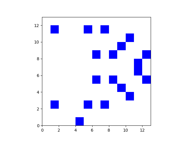
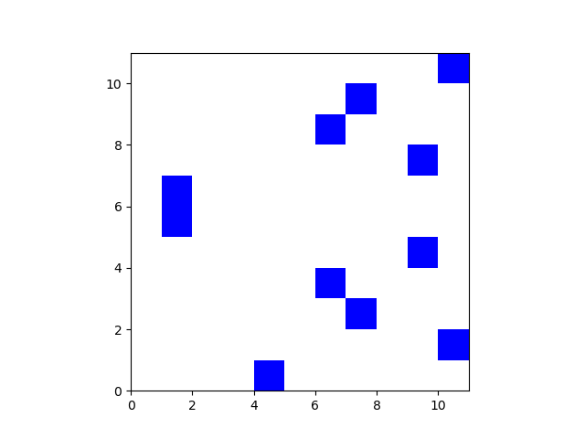
Here’s a checkerboard plot of TJJ, like the plots given here.

Note that there are 19 blue squares above. Elliptic curves always have an extra point at infinity not shown.

Montgomery form

One thing Tiny Jubjub has in common with the better known Jubjub curves is that it has a Montgomery form. That is, there is a change of variables that puts the curve in the form

By² = x³ + Ax + b

with B(A² − 4) ≠ 0. Every elliptic curve in Montgomery form can be put in Weierstrass form, but not vice versa; Montgomery curves are special.

TJJ can be put in Montgomery form with A = 6 and B = 7.

Twisted Edwards form

Every elliptic curve that can be put into Montgomery form can also be put into twisted Edwards form

a x² + y² = 1 + d x² y²

with a ≠ 0 ≠ d.

TJJ can be put into Montgomery form with a = 3 and d = 8.

It’s useful when a curve can be put in twisted Edwards form because elliptic curve arithmetic can be implemented without branching logic for special cases.

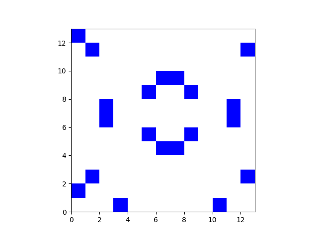
Note that this plot has 20 blue squares. That’s because for Montgomery curves, the point at infinity is (0, 1), and so it falls inside the grid we’re plotting.

SNARK friendly

TJJ is a SNARK-friendly curve, which is why it appears often in a book on zk-SNARKs. A curve is said to be SNARK friendly if in its twisted Edwards form a is a quadratic residue and d is not. In our case, that means

x² = 3 mod 13

has a solution but

x² = 8 mod 13

does not. We can verify this with the following Python code.

    >>> [x**2 % 13 for x in range(13)]
    [0, 1, 4, 9, 3, 12, 10, 10, 12, 3, 9, 4, 1]

Notice that 3 is in the output and 8 is not.

Related posts

Misleading plots of elliptic curves

The elliptic curves used in cryptography are over finite fields. They’re not “curves” at all in the colloquial sense of the word. But they are defined by analogy with continuous curves, and so most discussions of elliptic curves in cryptography start by showing a plot of a real elliptic curve.

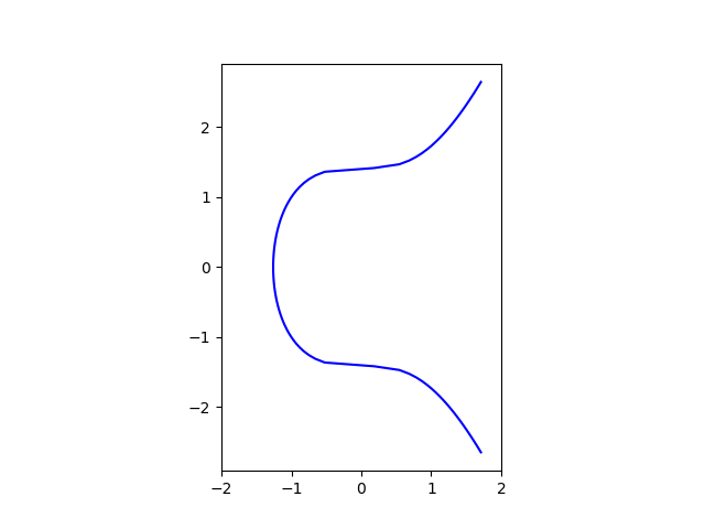
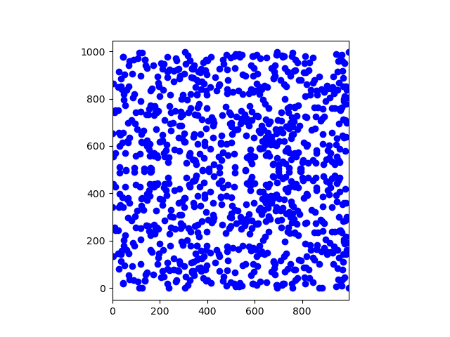
Here’s a plot of y² = x³ + 2 for real x and y.

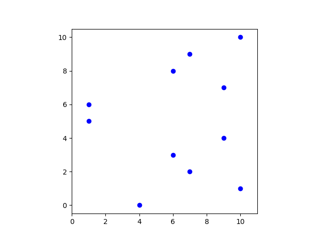
That’s fine as far as it goes. Resources quickly go on to say that the curves they’ll be looking at are discrete, and so they may then add something like the following. Here’s the same elliptic curve as above over the integers mod 11.

And again mod 997.

These plots are informative in a couple ways. First, they show that the elements of the curve are discrete points. Second, they show that the points are kinda randomly distributed, which hints at why elliptic curves might be useful in cryptography.

But the implied density of points is entirely wrong. It implies that the density of elliptic curve points increases with the field size increases, when in fact the opposite is true. The source of the confusion is using dots of constant size. A checkerboard graph would be better. Here’s a checkerboard plot for the curve mod 11.

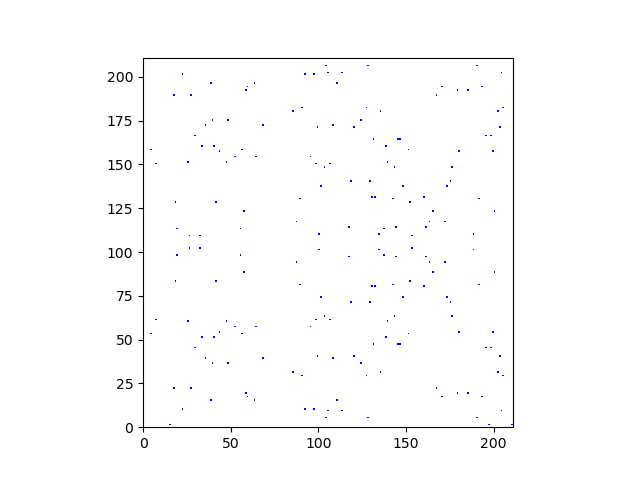
If we were to do the same for the curve mod 997 we’d see nothing. The squares would be too small and too few to see. Here’s a plot for the curve mod 211 that gives a hint of the curve elements as dust in the plot.

An elliptic curve over the integers modulo a prime p lives in a p by p grid, and the number of points satisfying the equation of an elliptic curve is roughly p. So the density of points in the grid that belong to the curve is 1/p.

The elliptic curves used in cryptography are over fields of size 2255 or larger, and so the probability that a pair of x and y values chosen at random would be on the curve is on the order of 2−255, virtually impossible.

We can be more precise than saying the number of points on the curve is roughly p. If p isn’t too large, we can count the number of points on an elliptic curve. For example, the curve

y² = x³ + 2 mod p

has 12, 199, and 988 points when p = 11, 211, and 997. (If you count the points in the plots above for p = 11 you’ll get 11 points. Elliptic curves always have an extra point at infinity not shown.)

Hasse’s theorem gives upper and lower bounds for the number of points N on an elliptic curve over a field of p elements with p prime:

|N − (p + 1)| ≤ 2 √p.

The heuristic for this is that the right hand side of the equation defining an elliptic curve

x³ + ax + b

is a square mod p above half the time. When it is a square, it corresponds to two values of y and when it is not it corresponds to zero points. So on average an elliptic curve mod p has around p ordinary points and one point at infinity.

Related posts

Counting points on an elliptic curve

Suppose you have an elliptic curve

y² = x³ + ax + b

over a finite field Fp for prime p. How many points are on the curve?

Brute force

You can count the number of points on the curve by brute force, as I did here. Loop through each of the p possibilities for x and for y and count how many satisfy the curve’s equation, then add one for the point at infinity. This is the most obvious but slowest approach, taking O(p²) time.

Here’s a slight variation on the code posted before. This time, instead of passing in the function defining the equation, we’ll assume the curve is in the form above (short Weierstrass form) and pass in the parameters a and b. This will work better when we refine the code below.

def order(a, b, p):
    c = 1 # The point at infinity
    for x in range(p):
        for y in range(p):
            if (y**2 - x**3 - a*x - b) % p == 0:
                c += 1
    return c

Better algorithm

A better approach would be to loop over the x values but not the y‘s. For each x, test determine whether

x³ + ax + b

is a square mod p by computing the Legendre symbol. This takes O(log³ p) time [1], and we have to do it for p different values of x, so the run time is O(p log³ p).

from sympy import legendre_symbol

def order2(a, b, p):
    c = 1 # The point at infinity
    for x in range(p):
        r = x**3 + a*x + b
        if r % p == 0:
            c += 1 # y == 0
        elif legendre_symbol(r, p) == 1:
            c += 2
    return c

Schoof’s algorithm

There’s a more efficient algorithm, Schoof’s algorithm. It has run time O(logk p) but I’m not clear on the value of k. I’ve seen k = 8 and k = 5. I’ve also seen k left unspecified. In any case, for very large p Schoof’s algorithm will be faster than the one above. However, Schoof’s algorithm is much more complicated, and the algorithm above is fast enough if p isn’t too large.

Comparing times

Let’s take our log to be log base 2; all logs are proportional, so this doesn’t change the big-O analysis.

If p is on the order of a million, i.e. around 220, then the brute force algorithm will have run time on the order of 240 and the improved algorithm will have run time on the order of 220 × 20³ ≈ 233. If k = 8 in Schoof’s algorithm, its runtime will be on the order of 208 ≈ 234, so roughly the same as the previous algorithm.

But if p is on the order of 2256, as it often is in cryptography, then the three algorithms have runtimes on the order of 2512, 2270, and 264. In this case Schoof’s algorithm is expensive to run, but the others are completely unfeasible.

[1] Note that logk means (log q)k, not log applied k times. It’s similar to the convention for sine and cosine.

Pairing-unfriendly curves

A couple days ago I wrote about two pair of closely related elliptic curves: Tweedledum and Tweedledee, and Pallas and Vesta.

In each pair, the order of one curve is the order of the base field of the other curve. The curves in each pair are used together in cryptography, but they don’t form a “pairing” in the technical sense of a bilinear pairing, and in fact none of the curves are “pairing-friendly” as described below.

An elliptic curve E/Fq is said to be pairing-friendly if r divides qk − 1 for some small k. Here r is the size of the largest prime-order subgroup of the curve, but since our curves have prime order p, r = p.

As for what constitutes a small value of k, something on the order of 10 would be considered small. The larger k is, the less pairing-friendly the curve is. We will show that our curves are extremely pairing-unfriendly.

Since q is not a multiple of p in our examples, there must be some power of q such at

qk = 1 mod p.

The question is whether k is large, i.e. whether the order of q mod p is large. We could try successive values of k, but that won’t get us very far. To be more clever, we use Lagrange’s theorem that says the order of an element divides the order of the group. So k must be one of the factors of p − 1. (We subtract 1 because we’re looking at the multiplicative group mod p, which removes 0.)

Finding the divisors of n − 1 requires factoring n − 1, which isn’t easy, but isn’t insurmountable either. The previous post reports the time required to do this in Python and in Mathematica for each of the following values of n.

p = 2254 + 4707489544292117082687961190295928833
q = 2254 + 4707489545178046908921067385359695873
r = 2254 + 45560315531419706090280762371685220353
s = 2254 + 45560315531506369815346746415080538113

Tweedledum has order p and its base field has order q.

k = 28948022309329048855892746252171976963322203655954433126947083963168578338816

Tweedledee has order q and its base field has order p.

k = 28948022309329048855892746252171976963322203655955319056773317069363642105856

Vesta has order r and its base field has order s.

k = 14474011154664524427946373126085988481681528240970780357977338382174983815168

Pallas has order s and its base field has order r.

k = 14474011154664524427946373126085988481681528240970823689839871374196681474048

It’s safe to say in each case k is not a small number.


Cycles of Elliptic Curves

The previous post gave two examples of pairs of elliptic curves in which

#(EFp) = q

and

#(EFq) = p.

That is, the curve E, when defined over integers mod p has q elements, and when defined over the integers mod q has p elements.

Pairs

Silverman and Stange [1] call this arrangement an amicable pair. They found a small pair of amicable elliptic curves:

y² = x³ + 2

with p and q equal to 13 and 19. They give many other examples, but this one is nice because it’s small enough for hand calculations, unlike the curves mentioned in the previous post that had on the order of 2254 elements.

Cycles

More generally, amicable curve pairs are amicable curve cycles with cycle length 3. Silverman and Stange give this example of a cycle of length 3:

y² = x³ − 25x − 8

with (p, q, r) = (83, 79, 73). That is, the curve over F83 has 79 elements, the curve over F79 has 73 elements, and the curve over F73 has 83 elements.

The authors show that there exist cycles of every length m ≥ 2.

Application

Why does any of this matter? Cycles of elliptic curves are useful in cryptography, specifically in zero-knowledge proofs. I hope to go into this further in some future post.

Confirmation

The curves mentioned above are small enough that we can compute the orders of the curves quickly by brute force. The following Python code confirms the claimed orders above.

def order(eqn, p):
    c = 1 # The point at infinity
    for x in range(p):
        for y in range(p):
            if eqn(x, y) % p == 0:
                c += 1
    return c

eqn = lambda x, y: y**2 - x**3 - 2
assert( order( eqn, 13) == 19 )
assert( order( eqn, 19) == 13 )

eqn = lambda x, y: y**2 - x**3 + 25*x + 8
assert( order( eqn, 83) == 79 )
assert( order( eqn, 79) == 73 )
assert( order( eqn, 73) == 83 )

Related posts

[1] Joseph H. Silverman and Katherine E. Stange. Amicable pairs and aliquot cycles for elliptic curves. Experimental Mathematics, 20(3):329–357, 2011.

Pallas, Vesta, and Zcash

Yesterday’s post mentioned Tweedledum and Tweedledee, a pair of elliptic curves named after characters in Lewis Carroll’s Through the Looking Glass.

Zcash uses a very similar pair of elliptic curves for zero-knowledge proofs: Pallas and Vesta. One named after a Greek goddess associated with war, and one named after a Roman goddess associated with home and hearth. (Zcash used the Jubjub curve, also mentioned yesterday, though not in the most recent release.)

The curves Pallas and Vesta are collectively known as the “pasta” curves, pasta being a portmanteau of pallas and vesta.

pa(llas ve)sta

Tweedledum, Tweedledee, Pallas, and Vesta all have the equation

y² = x³ + 5

over different prime-order fields.

The number of elements in Tweedledum’s field equals the number of elements in Tweedledee’s elliptic curve, and vice versa. The same relationship holds between Pallas and Vesta. And all four curves have roughly 2254 points.

If p is the size of Tweedledum’s field (and Tweedledee’s curve), and q is the size of Tweedledee’s field (and Tweedledum’s curve),

p = 2254 + 4707489545178046908921067385359695873
q = 2254 + 4707489544292117082687961190295928833

If p is the size of Pallas’ field (and Vesta’s curve), and q is the size of Vesta’s field (and Pallas’ curve),

p = 2254 + 45560315531419706090280762371685220353
q = 2254 + 45560315531506369815346746415080538113

Note that while Tweedledum and Tweedledee, and Pallas and Vesta, are “pairs” of curves used together, but they do not form a pairing in the technical sense of that word.