A few days ago I wrote about how to estimate 10^x. This is an analogous post for

exp(x) = e^x.

We will assume -0.5 ≤ x ≤ 0.5. You can bootstrap your way from there to other values of x. For example,

exp(1.3) = exp(1 + 0.3) = e exp(0.3)

and

exp(0.8) = exp(1 – 0.2) = e / exp(0.2).

I showed here that

log_e(x)≈ (2x − 2)/(x + 1)

for x between exp(-0.5) and exp(0.5).

Inverting both sides of the approximation shows

exp(x) ≈ (2 + x)/(2 − x)

for x between −0.5 and 0.5.

The maximum relative error in this approximation is less than 1.1% and occurs at x = 0.5. For x closer to the middle of the interval [−0.5, 0.5] the relative error is much smaller.

Here’s a plot of the relative error.

This was produced with the following Mathematica code.

    re[x_] := (Exp[x] - (2 + x)/(2 - x))/Exp[x]
    Plot[re[x], {x, -0.5, 0.5}]

Update: The approximations from this post and several similar posts are all consolidated here.

More approximation posts

• Simple trig function approximations
• Mentally calculating logarithms
• Why the log10 approximation is so simple

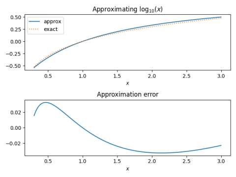
In my post on mentally calculating logarithms, I showed that

log₁₀ x ≈ (x − 1)/(x + 1)

for 1/√10 ≤ x ≤ √10. You could convert this into an approximation for logs in any base by multiplying by the right scaling factor, but why does it work out so simply for base 10?

Define

m(x) = (x − 1)/(x + 1).

Notice that m(1) = 0 and m(1/x) = −m(x), two properties that m shares with logarithms. This is a clue that there’s a connection between m and logs.

Now suppose we want to approximate log_b by k m(x) over the interval 1/√ b ≤ x ≤ √b. How do we pick k? If we choose

k = 1/(2m(√b))

then our approximation error will be zero at both ends of our interval.

If b = 10, k = 0.9625, i.e. close to 1. That’s why the approximation rule is particularly simple when b = 10. And although it’s good enough to round 0.9625 to 1 for rough calculations, our approximation for logs base 10 would be a little better if we didn’t.

More bases

In the process of asking why base 10 was special, we came up with a general way of constructing logarithm approximations for any base.

Using the method above we find that

log_e ≈ 2.0413 (x − 1)/(x + 1)

over the interval 1/√e ≤ x ≤ √e and that

log₂ ≈ 2.9142 (x − 1)/(x + 1)

over the interval 1/√2 ≤ x ≤ √2.

These rules are especially convenient if you round 2.0413 down to 2 and round 2.9142 up to 3. These changes are no bigger than rounding 0.9625 up to 1, which we did implicitly in the rule for logs base 10.

Curiosities

The log base 100 of a number is half the log base 10 of the number. So you could calculate the log of a number base 100 two ways: directly using b = 100 with the method above, or indirectly by setting b = 10 and dividing your result by 2. Do these give you the same answer? Nope! Our scaling is not linear in the (logarithm of) the base.

Well, then which is better? Taking the log base 10 first and dividing by 2 is better. In general, the smaller the base, the more accurate the result.

This seems strange at first, like something for nothing, but realize than when b is smaller, so is the interval we’re working over. You’ve done more work in reducing the range when you use a smaller base, and your reward is that you get a more accurate result. Since 2 is the smallest logarithm base that comes up with any regularity, the approximation for log base 2 is the most accurate of its kind that is likely to come up.

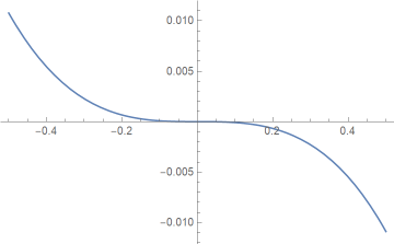
For every base b, we’ve shown that the approximation error is zero at 1/√b, 1, and √b. What we haven’t shown is that we have what’s known as “equal ripple” error. For example, here’s a plot of the error for our rule for approximating log base 2.

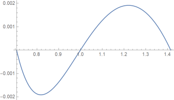
The error goes exactly as far negative on the left of 1 as it goes positive on the right of 1. The minimum is −0.00191483 and the maximum is 0.00191483. This follows from the property

m(1/x) = −m(x)

mentioned above. The location of the minimum (signed) error is the reciprocal location of the maximum error, and the value of that minimum is the negative of the maximum.

Update: The approximations from this post and several similar posts are all consolidated here.

This is the last in a sequence of three posts on mental calculation. The first looked at computing sine, cosine, and tangent in degrees. The second looked at computing logarithms, initially in base 10 but bootstrapping from there to other bases as well.

In the previous post, we showed that

log₁₀ x ≈ (x − 1)/(x + 1)

for x between 0.3 and 3.

If we take the inverse of the functions on both sides we get

10^x ≈ (1 + x)/(1 − x).

for x between −0.5 and 0.5.

If the fractional part of x is not between −0.5 and 0.5 use

10^{x + 0.5} = 10^x 10^0.5

to reduce it to that case.

For example, suppose you want a rough estimate of 10^2.7. Then

10^2.7 = 10² 10^0.5 10^0.2 ≈ 100 × 3 × 1.2/0.8 = 450

This calculation approximates the square root of 10 as 3. Obviously you’ll get a better answer if you use a better approximation for square root of 10. Incidentally, π is not a bad approximation to √10; using 3.14 would be better than using 3.

Plots and error

The graph below shows how good our approximation is. You can see that the error increases with x.

But the function we’re approximating also grows with x, and the relative error is nearly symmetric about zero.

Relative error is more important than absolute error if you’re going to multiply the result by something else, as we do when the fractional part of x has absolute value greater than 0.5.

Improvement

The virtue of the approximation above is that it is simple, and moderately accurate, with relative error less than 8%. If you want more accuracy, but still want something easy enough to calculate manually, a couple tweaks make the approximation more accurate.

The approximation

10^x ≈ (1 + x)/(1 − x)

is a little high on the left of zero, and a little low on the right. You can do a little better by using

10^x ≈ 0.95 (1 + x)/(1 − x)

for −0.5 < x < −0.1, and

10^x ≈ 1.05 (1 + x)/(1 − x)

for 0.1 < x < 0.5.

Now the relative error stays below 0.03. The absolute error is a little high on the right end, but we’ve optimized for relative error.

In case you’re wondering where the factors of 0.95 and 1.05 came from, they’re approximately 3/√10 and √10/3 respectively.

Update: The approximations from this post and several similar posts are all consolidated here.

The previous post looked at approximations for trig functions that are simple enough to compute without a calculator. I wondered whether I could come up with something similar for logarithms. I start with log base 10. Later in the post I show how to get to find logs in other bases from logs base 10.

Let

x = m × 10^p.

where 1 ≤ m ≤ 10. Then

log₁₀(x) = log₁₀(m) + p

and so without loss of generality we can assume 1 ≤ x ≤ 10.

But we can narrow our range a little more. If x > 3, compute the log of x‘ = x/10, and if x < 0.3 then compute the log of 10x. So we will assume

0.3 ≤ x ≤ 3.

For x in this range

log₁₀(x) ≈ (x − 1)/(x + 1)

is a remarkably good approximation. The absolute error is less than 0.0327 on the interval [0.3, 3].

Examples

log₁₀ 0.6 ≈ (0.6 − 1)/(0.6 + 1) = −1/4 = −0.25. Exact: −0.2218

log₁₀ 1776 = 3 + log₁₀ 1.776 ≈ 3 + 0.776/2.776 = 3.2795. Exact: 3.2494

log₁₀ 9000 = 4 + log₁₀ 0.9 ≈ 4 − 0.1/1.9 = 3.9473. Exact: 3.9542

Other bases

Logs to all bases are proportional, so you can convert between log base 10 and log to any other base by multiplying by a proportionality constant.

log_b(x) = log₁₀(x) / log₁₀(b).

So suppose, for example, you want to compute log₂ 48. Since 48 = 32 × 1.5 we have

log₂ 48 = log₂ 32 + log₂ 1.5 = 5 + log₁₀ 1.5 / log₁₀ 2

We can approximate log₁₀ 1.5 as 1/5 and log₁₀ 2 as 1/3 to get

log₂ 48 = 5 + 3/5 = 5.6.

The exact value is 5.585.

If you want to use this for natural logs, you might want to memorize

1/log₁₀ e = log_e 10 = 2.3.

Update: There’s a better way to work with other bases. See this post. The same post explains why the approximation is particularly simple for logs base 10.

More accuracy

Abramowitz and Stegun refines the approximation t = (x − 1)/(x + 1). They use the interval [1/√10, √10] rather than [0.3, 3]. This slightly different interval is symmetric about 0 when you convert to t. Equation 4.1.41 runs t through a cubic polynomial and lowers the absolute error to less than 6 × 10⁻⁴. Equation 4.1.42 uses a 9th degree polynomial in t to lower the absolute error below 10⁻⁹.

Next

My next post will show how to compute 10^x analogously.

Related posts

• Simple approximations for trig functions in degrees
• Simple approximation for normal probabilities
• Memorizing numbers
• Mentally computing scientific calculator functions.

Anthony Robin gives three simple approximations for trig functions in degrees in [1].

The following plots show that these approximations are pretty good. It’s hard to distinguish the approximate and exact curves.

The accuracy of the approximations is easier to see when we subtract off the exact values.

The only problem is that the tangent approximation is poor for small angles [2]. The ratio of the sine and cosine approximations makes a much better approximation, but it this requires more work to evaluate. You could use the ratio for small angles, say less than 20°, and switch over to the tangent approximation for larger angles.

Update: The approximations from this post and several similar posts are all consolidated here.

Here’s the Python code that was used to create the plots in this post. It uses one trick you may find interesting, using the eval function to bridge between the names of functions and the functions themselves.

from numpy import sin, cos, tan, linspace, deg2rad
import matplotlib.pyplot as plt

sin_approx = lambda x: 0.01*x*(2-0.01*x)
cos_approx = lambda x: 1 - x*x/7000.0
tan_approx = lambda x: (10.0 + x)/(100.0 - x)

trig_functions = ["sin", "cos", "tan"];
x = linspace(0, 45, 100)

fig, ax = plt.subplots(3,1)
for n, trig in enumerate(trig_functions):
    ax[n].plot(x, eval(trig + "_approx(x)"))
    ax[n].plot(x, eval(trig + "(deg2rad(x))"), ":")
    ax[n].legend(["approx", "exact"])
    ax[n].set_title(trig)
    ax[n].set_xlabel(r"$x\degree$")

plt.tight_layout()
plt.savefig("trig_approx_plot.png")

fig, ax = plt.subplots(3,1)
for n, trig in enumerate(trig_functions):
    y = eval(trig + "_approx(x)")
    z = eval(trig + "(deg2rad(x))")
    ax[n].plot(x, y-z)
    ax[n].set_title(trig + " approximation error")
    ax[n].set_xlabel(r"$x\degree$")

plt.tight_layout()
plt.savefig("trig_approx_error.png")

tan_approx2 = lambda x: sin_approx(x)/cos_approx(x)

fig, ax = plt.subplots(2, 1)
y = tan(deg2rad(x))
ax[0].plot(x, tan_approx2(x))
ax[0].plot(x, y, ":")
ax[0].legend(["approx", "exact"], loc="lower right")
ax[0].set_title("Ratio of sine and cosine approx")
ax[1].plot(x, y - tan_approx(x), "-")
ax[1].plot(x, y - tan_approx2(x), "--")
ax[1].legend(["direct approx", "ratio approx"])
ax[1].set_title("Approximation errors")

plt.tight_layout()
plt.savefig("tan_approx.png")

Related posts

• Calculating normal probabilities with a simple calculator
• Trig functions across programming languages

[1] Anthony C. Robin. Simple Trigonometric Approximations. The Mathematical Gazette, Vol. 79, No. 485 (Jul., 1995), pp. 385-387

[2] When I first saw this I thought “No big deal. You can just use tan θ ≈ θ for small angles, or tan θ ≈ θ + θ³/3 if you need more accuracy.” But these statements don’t apply here because we’re working in degrees, not radians.

tan θ° is not approximately θ for small angles but rather approximately π θ / 180. If you’re working without a calculator you don’t want to multiply by π if you don’t have to, and a calculator that doesn’t have keys for trig functions may not have a key for π.

A couple years ago I wrote about a trick for mentally computing the fifth root of an integer if you know that the number you’re starting with is the fifth power of a two-digit number.

This morning I wrote up a similar (and simpler) trick for cube roots as a thread on @AlgebraFact. You can find the Twitter thread starting here, or you could go to this page that unrolls the whole thread in one page.