I’ve written several posts about using Claude or ChatGPT to generate Prolog or Lean code to solve a chess puzzle. I didn’t think Grok would be up to the task, though I didn’t try it. I’ve heard good things about Grok 4.5, so I gave it a shot. It did great.
Here’s the problem, a variation on the n-queens problem formulated by Martin Gardner.
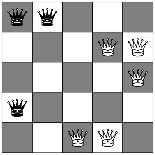
Can you place five white queens and three black queens on a 5 × 5 board so that no queen of one color attacks a queen of another color?
Here’s the prompt I have Grok 4.5.
Generate SWI Prolog code to solve the following chess puzzle. On a 5 by 5 chessboard, place 5 white queens and 3 black queens so that no queen is attacking a queen of the other color. Have the code enumerate all solutions.
The code ran correctly, giving all eight solutions.
I then asked Grok
Now generate Lean 4 code to solve the same puzzle.
The code did not run on the first or second attempts but ran correctly on the third iteration. That’s better than I’ve seen before. It’s not an apples-to-apples comparison, but it has usually taken many iterations with Claude before Lean code would run.
Solutions
There are eight solutions, each being a flip or a rotation of one fundamental solution. Here’s a representative.
SWI Prolog code
:- use_module(library(clpfd)).

%% Enumerate all ways to place 5 white queens and 3 black queens
%% on a 5x5 board so that no queen attacks a queen of the opposite colour.
%% Same-colour queens are allowed to attack each other.
%%
%% Positions are numbered 1..25 in row-major order:
%%   1  2  3  4  5
%%   6  7  8  9 10
%%  11 12 13 14 15
%%  16 17 18 19 20
%%  21 22 23 24 25

solve :-
    solution(Whites, Blacks),
    print_solution(Whites, Blacks),
    fail.
solve :-
    writeln('No more solutions.').

solution(Whites, Blacks) :-
    length(Whites, 5),
    length(Blacks, 3),
    append(Whites, Blacks, All),
    All ins 1..25,
    all_distinct(All),
    % canonical order so each set of positions is generated once
    Whites = [W1,W2,W3,W4,W5],
    W1 #< W2, W2 #< W3, W3 #< W4, W4 #< W5,
    Blacks = [B1,B2,B3],
    B1 #< B2, B2 #< B3, % every black is safe from every white maplist(safe_from_all(Whites), Blacks), label(All). safe_from_all(Whites, Black) :- maplist(no_attack(Black), Whites). %% Two queens do *not* attack each other. no_attack(P, Q) :- R1 #= (P-1) div 5 + 1, C1 #= (P-1) mod 5 + 1, R2 #= (Q-1) div 5 + 1, C2 #= (Q-1) mod 5 + 1, R1 #\= R2, % different row C1 #\= C2, % different column abs(R1-R2) #\= abs(C1-C2). % different diagonal print_solution(Whites, Blacks) :- format('Whites: ~w~n', [Whites]), format('Blacks: ~w~n', [Blacks]), forall(between(1, 5, R), ( forall(between(1, 5, C), ( Pos is (R-1)*5 + C, ( memberchk(Pos, Whites) -> write('W ')
                      ; memberchk(Pos, Blacks) -> write('B ')
                      ; write('. ')
                      )
                    )),
             nl )),
    nl.
Lean 4 code
-- Lean 4 solution for the 5×5 black-and-white queens puzzle.
-- 5 white queens + 3 black queens; no opposite-colour attacks.

def absDiff (a b : Nat) : Nat :=
  if a ≥ b then a - b else b - a

def attacks (p q : Nat × Nat) : Bool :=
  p.1 == q.1 || p.2 == q.2 || absDiff p.1 q.1 == absDiff p.2 q.2

/-- All 25 squares (0-based, row-major). -/
def allPositions : List (Nat × Nat) :=
  (List.range 5).flatMap fun r =>
    (List.range 5).map fun c => (r, c)

/-- Combinations of length exactly `k` (order-preserving). -/
def combinations {α : Type} : Nat → List α → List (List α)
  | 0,     _      => [[]]
  | _,     []     => []
  | k + 1, x::ys  =>
      (combinations k ys).map (fun zs => x :: zs) ++
      combinations (k + 1) ys

def isAttackedBy (pos : Nat × Nat) (queens : List (Nat × Nat)) : Bool :=
  queens.any (fun q => attacks q pos)

/-- Every solution as a pair (white squares, black squares). -/
def solve : List (List (Nat × Nat) × List (Nat × Nat)) :=
  (combinations 3 allPositions).foldl (fun acc blacks =>
    let forbidden := allPositions.filter fun p =>
      blacks.contains p || isAttackedBy p blacks
    let available := allPositions.filter fun p =>
      !(forbidden.contains p)
    acc ++ (combinations 5 available).map fun whites => (whites, blacks)
  ) []

/-- Pretty-print one board. -/
def printBoard (whites blacks : List (Nat × Nat)) : IO Unit := do
  for r in List.range 5 do
    let mut row := ""
    for c in List.range 5 do
      let p := (r, c)
      row := row ++
        (if whites.contains p then "W "
         else if blacks.contains p then "B "
         else ". ")
    IO.println row
  IO.println ""

/-- Enumerate and display every solution. -/
def main : IO Unit := do
  let sols := solve
  IO.println s!"Found {sols.length} solutions.\n"
  for p in (List.range sols.length).zip sols do
    let i := p.1
    let (whites, blacks) := p.2
    IO.println s!"Solution {i + 1}:"
    printBoard whites blacks

#eval main