I just heard about PolyMon this evening. It’s an open source system monitoring project. It can monitor servers, system logs, etc. Users can create custom monitors via PowerShell scripts. Sounds like its worth further investigation.
Update: Link rot
I just heard about PolyMon this evening. It’s an open source system monitoring project. It can monitor servers, system logs, etc. Users can create custom monitors via PowerShell scripts. Sounds like its worth further investigation.
Update: Link rot
Textbooks say the normal approximation to the binomial distribution is good when “n is large.” How large is large enough? Some books say n ≥ 10. How good is it in that case? Hmm, it doesn’t say. The same holds for the normal approximation to the Poisson. The only advice you’re likely to see is that the approximation is better when the λ parameter is “large.”
Approximations are much more useful when you have an error bound or an error estimate, and yet I’ve never seen a textbook that gave an error bound when introducing these approximations. You’ll probably get an example or two, but nothing general. One justification for this omission is that the error bounds rely on more advanced results than could be proven in an introductory class. But the approximation result is already a rabbit out of a hat. Why not pull one more rabbit out of the hat and state an error bound?
I’m supposed to teach a math stat class in the Fall. I’ve prepared some notes looking into the details of the various approximations so I could do better than just wave my hands when presenting this material. Here are my notes for the Poisson and binomial distributions.
Here’s one of the graphs from the notes, an example showing the error in normal approximation to a Poisson(20) density function.
E. Kowalski has a post this morning called Finding life beyond the Central Limit Theorem. The post mentions a theorem I’ve never heard of that connects basic concepts in probability and number theory.
Surely the Central Limit Theorem and the normal distribution are important in probability. You might even call them “central.” And counting prime divisors of integers is a natural thing to do in number theory. It turns out these two concepts are closely related.
Pick a big number N. Now select a random integer n between 1 and N. Count the number of distinct prime divisors of n and call that ω(n). Roughly speaking, ω(n) acts like a normal random variable with mean and variance log log N.
There are plenty of other connections between probability and number theory. I took probability from Jeffrey Vaaler, a number theorist. I remember three informal remarks he made to suggest connections between number theory and probability.
Classroom exercises always have nice, tidy solutions. So students implicitly assume that all problems have nice, tidy solutions. If the solution isn’t working out simply, you must have made a mistake.
Outside the classroom, applications seldom have simple solutions. So after a while you get jaded and quit trying to find a simple solution. But sometimes real problems do have simple solutions, or at least simpler solutions than seemed possible.
The Extreme Programming folks have a saying “Try the simplest thing that could possibly work.” If that doesn’t work, then try the next simplest thing that could possibly work. That line of thinking has paid off a few times lately.
I’ve had a couple math problems that I first assumed had to be approximated numerically that were more easily computed exactly. And I’ve had a couple programs where I was able to debug a section of code by simply deleting it. Things don’t always work out that well, but it’s fun when they do.
Jeff Atwood’s latest post asks whether money useless to open source projects. Four months after his donation of $5,000 to the ScrewTurn Wiki project, they haven’t cashed his check because they haven’t thought of a way to use the money even though Jeff placed absolutely no restrictions on what they could do with it.
Jeff concludes that there’s something about open source projects that makes it harder for them to spend money. But I’ve seen the same thing outside of the open source world. I’ve often had people tell me they want a job done and offer me some chunk of grant money. The grant money would not be enough to hire a new developer on salary, and the funds couldn’t be used to hire a contractor. Either the job was too small to outsource or there was a legal restriction on how the money could be used. The project would just be extra work for the staff we already have and the grant money would be useless to the people doing the work.
My previous post listed seven things that cause new brain cells to grow, taken from a talk by Dean Ornish (link died). Here’s the corresponding list from the same talk of things that decrease brain cells.
Dr. Dean Ornish gave an inspiring three-minute talk at TED entitled Your genes are not your fate. As part of his talk he lists six things that cause new brain cells to grow:
The first post in this series introduced random inequalities. The second post discussed random inequalities can could be computed in closed form. This post considers random inequalities that must be evaluated numerically.
The simplest and most obvious approach to computing P(X > Y) is to generate random samples from X and Y and count how often the sample from X is bigger than the sample from Y. However, this approach is only accurate on average. In any particular sample, the error may be large. Even if you are willing to tolerate, for example, a 5% chance of being outside your error tolerance, the required number of random draws may be large. The more accuracy you need, the worse it gets since your accuracy only improves as n−1/2 where n is the number of samples. For numerical integration methods, the error decreases as a much larger negative power of n depending on the method. In the timing study near the end of this technical report, numerical integration was 2,875 times faster than simulation for determining beta inequality probabilities to just two decimal places. For greater desired accuracy, the advantage of numerical integration would increase.
Why is efficiency important? For some applications it may not be, but often these random inequalities are evaluated in the inner loop of a simulation. A simulation study that takes hours to run may be spending most of its time evaluating random inequalities.
As derived in the previous post, the integral to evaluate is given by
![\begin{eqnarray*} P(X \geq Y) &=& \int \!\int _{[x > y]} f_X(x) f_Y(y) \, dy \, dx \\ &=& \int_{-\infty}^\infty \! \int_{-\infty}^x f_X(x) f_Y(y) \, dy \, dx \\ &=& \int_{-\infty}^\infty f_X(x) F_Y(x) \, dx end{eqnarray*}](http://www.johndcook.com/ineq_integral.svg)
The technical report Numerical computation of stochastic inequality probabilities gives some general considerations for numerically evaluating random inequalities, but each specific distribution family must be considered individually since each may present unique numerical challenges. The report gives some specific techniques for beta and Weibull distributions. The report Numerical evaluation of gamma inequalities gives some techniques for gamma distributions.
Numerical integration can be complicated by singularities in integrand for extreme values of distribution parameters. For example, if X ~ beta(a, b) the integral for computing P(X > Y) has a singularity if either a or b are less than 1. For general advice on numerically integrating singular integrands, see “The care and treatment of singularities” in Numerical Methods that Work by Forman S. Acton.
Once you come up with a clever numerical algorithm for evaluating a random inequality, you need to have a way to test the results.
One way to test numerical algorithms for random inequalities is to compare simulation results to integration results. This will find blatant errors, but it may not be as effective in uncovering accuracy problems. It helps to use random parameters for testing.
Another way to test numerical algorithms in this context is to compute both P(X > Y) and P(Y > X). For continuous random variables, these two values should add to 1. Of course such a condition is not sufficient to guarantee accuracy, but it is a simple and effective test. The Inequality Calculator software reports both P(X > Y) and P(Y > X) partly for the convenience of the user but also as a form of quality control: if the two probabilities do not add up to approximately 1, you know something has gone wrong. Along these lines, it’s useful to verify that P(X > Y) = 1/2 if X and Y are identically distributed.
Finally, integrands may have closed-form solutions for special parameters. For example, Exact calculation of beta inequalities gives closed-form results for many special cases of the parameters. As long as the algorithm being tested does not depend on these special values, these special values provide valuable test cases.
My previous post introduced random inequalities and their application to Bayesian clinical trials. This post will discuss how to evaluate random inequalities analytically. The next post in the series will discuss numerical evaluation when analytical evaluation is not possible.
For independent random variables X and Y, how would you compute P(X>Y), the probability that a sample from X will be larger than a sample from Y? Let fX be the probability density function (PDF) of X and let FX be the cumulative distribution function (CDF) of X. Define fY and FY similarly. Then the probability P(X > Y) is the integral of fX(x) fY(y) over the part of the x–y plane below the diagonal line x = y.
This result makes intuitive sense: fX(x) is the density for x and FY(x) is the probability that Y is less than x. Sometimes this integral can be evaluated analytically, though in general it must be evaluated numerically. The technical report Numerical computation of stochastic inequality probabilities explains how P(X > Y) can be computed in closed form for several common distribution families as well as how to evaluate inequalities involving other distributions numerically.
Exponential: If X and Y are exponential random variables with mean μX and μY respectively, then
P(X > Y) = μX/(μX + μY).
Normal: If X and Y are normal random variables with mean and standard deviation (μX, σX) and (μY, σY) respectively, then
P(X > Y) = Φ((μX − μY)/√(σX2 + σY2))
where Φ is the CDF of a standard normal distribution.
Gamma: If X and Y are gamma random variables with shape and scale (αX, βX) and (αY, βY) respectively, then
P(X > Y) = Ix(βX/(βX + βY))
where Ix is the incomplete beta function with parameters αY and αX, i.e. the CDF of a beta distribution with parameters αY and αX.
The inequality P(X > Y) where X and Y are beta random variables comes up very often in applications. This inequality cannot be computed in closed form in general, though there are closed-form solutions for special values of the beta parameters. If X ~ beta(a, b) and Y ~ beta(c, d), the probability P(X > Y) can be evaluated in closed form if
These last two cases can be combined with a recurrence relation to compute other probabilities. See Exact calculation of beta inequalities for more details.
Sometimes you need to calculate P(X > max(Y, Z)) for three independent random variables. This comes up, for example, when computing adaptive randomization probabilities for a three-arm clinical trial. For a time-to-event trial as implemented here, the random variables have a gamma distribution. See Numerical evaluation of gamma inequalities for analytical as well as numerical results for computing P(X > max(Y, Z)) in that case.
The next post in this series will discuss how to evaluate random inequalities numerically when closed-form integration is not possible.
Update: See Part IV of this series for results with the Cauchy distribution.
Many Bayesian clinical trial methods have at their core a random inequality. Some examples from M. D. Anderson: adaptive randomization, binary safety monitoring, time-to-event safety monitoring. These methods depend critically on evaluating P(X > Y) where X and Y are independent random variables. Roughly speaking, P(X > Y) is the probability that the treatment represented by X is better than the treatment represented by Y. In a trial with binary outcomes, X and Y may be the posterior probabilities of response on each treatment. In a trial with time-to-event outcomes, X and Y may be posterior probabilities of median survival time on two treatments.
People often have a little difficulty understanding what P(X > Y) means. What does it mean? If we take a sample from X and a random sample from Y, P(X >Y) is the probability that the former is larger than the latter. Most confusion around random inequalities comes from thinking of random variables as constants, not random quantities. Here are a couple examples.
First, suppose X and Y have normal distributions with standard deviation 1. If X has mean 4 and Y has mean 3, what is P(X > Y)? Some would say 1, because X is bigger than Y. But that’s not true. X has a larger mean than Y, but fairly often a sample from Y will be larger than a sample from X. P(X > Y) = 0.76 in this case.
Next, suppose X and Y are identically distributed. Now what is P(X > Y)? I’ve heard people say zero because the two random variables are equal. But they’re not equal. Their distribution functions are equal but the two random variables are independent. P(X > Y) = 1/2 by symmetry.
I believe there’s a psychological tendency to underestimate large inequality probabilities. (I’ve had several discussions with people who would not believe a reported inequality probability until they computed it themselves. These discussions are important when the decision whether to continue a clinical trial hinges on the result.) For example, suppose X and Y represent the probability of success in a trial in which there were 17 successes out of 30 on X and 12 successes out of 30 on Y. Using a beta distribution model, the density functions of X and Y are given below.
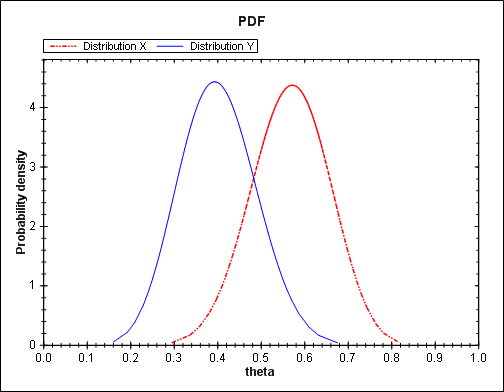
The density function for X is essentially the same as Y but shifted to the right. Clearly P(X > Y) is greater than 1/2. But how much greater than a half? You might think not too much since there’s a lot of mass in the overlap of the two densities. But P(X > Y) is a little more than 0.9.
The image above and the numerical results mentioned in this post were produced by the Inequality Calculator software.
Part II will discuss analytically evaluating random inequalities. Part III will discuss numerically evaluating random inequalities.