Sometimes it’s right under your nose

Neptune was discovered in 1846. But Galileo’s notebooks describe a “star” he saw on 28 December 1612 and 2 January 1613 that we now know was Neptune. Galileo even noticed that his star was in a slightly different location for his two observations, but he chalked the difference up to observational error.

The men who discovered Neptune were not the first to see it; they were the first to realize what they were looking at.

Three ways to convert documents to PDF

Microsoft has an Office 2007 plug-in that lets you save documents as PDF files. This works for all Microsoft Office applications, not just Microsoft Word. The only drawback is that this only works for Office 2007, not earlier versions of Office, and does not work with other document types.

Adobe Acrobat (not the free Adobe Reader) installs a printer driver that lets you convert any document to a PDF by “printing” it to their software. The advantage is that this works for any document type. However, if you’re starting with a Word 2007 document, Microsoft’s plug-in is much faster, maybe 10x faster.

If you don’t want to buy Adobe Acrobat, you could use PDF995. Like Adobe Acrobat, this installs a printer driver; you convert documents to PDF by choosing this software as your “printer.” PDF995 comes in two versions: a free version supported by advertising, and an advertising-free version for $9.95.

I would rank these methods in the order presented above. I’ve had the best experience with the Microsoft plug-in. The Acrobat printer driver is slow, but usually does a good job. The PDF995 printer driver works OK most of the time, but I had a few issues with it. It’s been a long time since I used it, but I think the problems had to do with unwanted footers and sometimes fonts in the PDF not matching the original fonts. I’m not sure now, but I think I’ve also had problems with the Acrobat printer driver.

If you want to make a PDF from a LaTeX document, use the pdflatex program that ships with LaTeX. I’ve never had any problems with it.

Update: See this post for notes on PDFCreator and pdftk.

Experimenting with Out-Speech in PowerShell

I’ve played around with the PSCX script Out-Speech at home and at work. At home, running Vista, words come out in a natural female voice. At work, running XP, words come out in a robotic male voice.

The voice is somewhat configurable. I didn’t try it at home, but at work I opened the Speech Properties applet in the control panel. All three are mechanical voices. I went to Microsoft’s website to see if I could download a natural voice. The site said that Microsoft does not provide other voices but it gives a link to third party providers.

My guess is that Microsoft deliberately put lame voices in XP for fear of a lawsuit and that they were braver by the time Vista was released.

Another difference I noticed between Vista and XP is tolerance of misspellings. XP will correctly pronounce “Fahrenheit” but pronounces the incorrect “Farenheit” so that it rhymes with “heat” rather than “height”. Vista correctly pronounces the misspelled word.

Testing and getting nowhere

Suppose a Martian gives you a black box. It has a button on top and a display on the side. Every time you press the button, the box displays a number. You want to figure out the pattern to the numbers, so you make a record of the outputs and keep a running average. You hit the button 100 times, but the average keeps moving around. So you decide to keep going until you’ve hit the button 1000 times. The average still doesn’t seem to be settling on a particular value.

Cumulative sample average of samples from a Cauchy(3,1) distribution

What kind of devilish box has the Martian given you? It’s a Cauchy random number generator. Here’s how you could make your own.

  1. Generate a random number uniformly between 0 and 1
  2. Subtract 0.5
  3. Multiply by π
  4. Take the tangent
  5. Add a constant
  6. Print the result
  7. Go back to 1

If you ever suspect that you’re in possession of a black box with a Cauchy random number generator inside, keep a running median of your samples rather than a running average. The running average will never converge.

See Cauchy distribution parameter estimation for more graphs and more explanation.

Index of tail weight in statistics

Ever since Chris Anderson started writing about the long tail, there has been popular interest in “tails.” Popular writers like Chris Anderson don’t use statistical jargon, but what they call the “tail” is the tail of a statistical distribution. Some distributions have “thick” or “heavy” tails, meaning that they approach zero slowly in the extremes. Other distributions have “thin” or “light” tails, meaning the approach zero quickly.

This morning I ran across a new way of measuring how thick the tail of a distribution is. It’s called “index of tail weight.” If F(x) is the distribution (CDF) function of a random variable, the index of tail weight is defined as

\tau(F) = \frac{F^{-1}(0.99) - F^{-1}(0.50)}{F^{-1}(0.75) - F^{-1}(0.50)} \left/ \frac{\Phi^{-1}(0.99) - \Phi^{-1}(0.50)}{\Phi^{-1}(0.75) - \Phi^{-1}(0.50)}\right.<br />

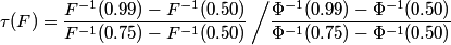
where Φ is the distribution function of a standard normal. In words, this formula says to calculate the difference between the 99th percentile and the median and divide by the difference between the 75th percentile and the median for your distribution. Then divide by the same ratio for a normal distribution. This means that the index of tail weight will be 1 for a normal distribution. A little calculation shows that the definition is independent of location and scale for a location-scale family of distributions. So, for example, the index of tail weight will be 1 for any normal distribution, not just a standard normal.

bar chart of tail thickness for several distributions

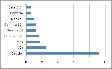
I’ve played around with this definition a little, and it seems to behave as I’d expect. The Cauchy distribution has a large index, 9.22588, and most distributions have smaller values.

For a gamma distribution, the index is independent of scale but depends on shape. A gamma with shape 1 (i.e. an exponential distribution) has weight 1.63635. As the shape increases, the index decreases, approaching 1 for large shape values. This makes sense because the gamma distribution becomes more like the normal as the shape parameter increases.

For the Student-t distribution, the index decreases to 1 as the degrees of freedom increase. This is what you’d expect since the t becomes approximately normal for large degrees of freedom.

The Weibull distribution has a larger index of tail weight than an exponential when the shape parameter is small, and the index decreases as the shape increases. For shape parameter 4, the Weibull has index 0.927819, which is reasonable since the tail then the tail falls off like exp(−x4) while the normal falls off like exp(-x2).

The book I found the definition in was Understanding Robust and Exploratory Data Analysis.

More heavy tail posts