Whatever happened to data modeling?

Posted on 14 February 2009 by John

Check out Michael Duffy’s new post Where Have All The Data Modelers Gone?

Data modeling used to be a valued specialization. Then Moore’s Law let companies worry less about data storage efficiency. Developers would do their own database designs, often with little regard for efficiency. Some companies have always cared about data modeling, but fewer over time. But that trend may be reversing. Now that companies are storing rapidly increasing volumes of data, there area new opportunities for data modelers to be heroes.

(Data storage is literally growing exponentially for now. One of my pet peeves is people saying that something is growing exponentially when that’s not what they mean. But in this case, the term is justified.)

Old math books

Posted on 14 February 2009 by John

In a previous post I quoted C. S. Lewis on the value of reading old books. He argued that every generation has its blind spots, and one way to see past the contemporary blind spots is to read old books. In that spirit, here are some of my favorite old math books.

Inequalities by Hardy, Littlewood, and Pólya. First published in 1934, second edition 1952.
A course in modern analysis by Whittaker and Watson. First published 1902, fourth edition 1927.
An Introduction to Probability Theory and Its Applications by William Feller. First edition 1950, third edition 1968.

These books contain useful facts hard to find elsewhere. More importantly, they embody an approach to mathematics that has fallen out of fashion. I believe the latter is what Lewis had in mind, not merely reference books but books that encapsulate the perspective of an earlier generation.

Don’t try to be God, try to be Shakespeare

Posted on 12 February 2009 by John

Here’s a quote from Twyla Tharp’s book The Creative Habit.

Honey, it’s all been done before. Nothing’s really original. Not Homer or Shakespeare and certainly not you. Get over yourself.

Trying to be completely original is paralyzing, and not even possible. Only God creates ex nihilo. Everyone else starts with something. Don’t try to be God. Try to be Homer or Shakespeare.

Related post: Three quotes on originality

Sums of uniform random values

Posted on 12 February 2009 by John

Suppose you have uniform random samples from the interval [0, 1]. If you add a large number of such samples together, the sum has an approximately normal distribution according to the central limit theorem. But how many do you have to add together to get a good approximation to a normal? Well, two is clearly not enough. Here’s what the density looks like for the sum of two uniform values.

But look what happens when we add three uniforms together. If you’re very familiar with the normal distribution and have a good eye, you might be able to tell that the density is a little flat at the top.

Here’s a graph that shows the distribution for a sum of four uniforms. The dotted curve is the graph of the normal distribution with the same mean and variance as the sum of the four uniforms. If the two graphs were not on top of each other, hardly anyone could tell which was the normal and which was the sum of uniforms.

Note that this fast convergence to a normal distribution is a special property of uniform random variables. The sum of four exponential random variables, for example, does not look nearly so normal.

Here’s the analytic expression for the density of the sum of n uniform random variables that was used to produce these graphs.

$\frac{1}{(n-1)!} \sum_{k=0}^n (-1)^k {n \choose k} (x-k)_+^{n-1}$

Here the notation z₊ stands for the positive part of z, i.e. the expression z₊ equals z if z is positive and equals 0 otherwise.

According to Feller’s classic book, the density result above was discovered by Lagrange. Feller gives a series of exercises leading up to this result. First he gives the distribution function for the sum of n-sided dice and asks the reader to prove the result. Then the reader is asked to take the limit as the number of sides on each dice goes to infinity to derive the result for uniform random variables.

John Venier left a comment to a previous post about the following method for generating a standard normal: add 12 uniform random variables and subtract 6. Note that this is not just any normal distribution but a standard normal, i.e. mean 0 and variance 1. Since the variance of a single uniform random variable is 1/12, adding 12 such values makes the variance 1. How good is the generator he describes? The maximum difference between the CDF of his generator and the CDF of a standard normal is about 0.00234.

Related post: Rolling dice for normal samples

Best early blog posts

Posted on 10 February 2009 by John

Here are some of the best posts by category from the first month of this blog.

PowerShell A-Z series completed

Posted on 10 February 2009 by John

Joe Pruitt has finished his PowerShell A-Z series.

Rolling dice for normal samples

Posted on 10 February 2009 by John

Roll five dice and use the sum to simulate samples from a normal distribution. This is an idea I ran across in Teaching Statistics by Andrew Gelman and Deborah Nolan. The book mentions this idea in the context of a classroom demonstration where students are to simulate IQ scores.

I was surprised that just five dice would do a decent job. So just how good a job does the dice generator do?

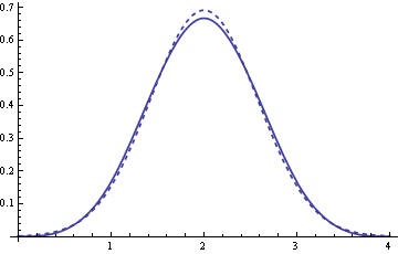
To find out, I looked at the difference between the cumulative densities of the dice generator and an exact normal generator. When you roll a single six-sided die, the outcomes have mean 3.5 and variance 35/12, and so the corresponding mean and variance for rolling 5 dice is 5 times greater. By the central limit theorem, the sum of the five rolls should have approximately the same distribution as a normal random variable with the same mean and variance. So what we want to do is compare the distribution of the sum of the five dice rolls to a Normal(17.5, 3.819²).

Now how do we get the distribution of the sum of the five dice? For one die it’s easy: the numbers 1 through 6 all have probability 1/6 of showing up. The sum of two dice is harder, but not too hard to brute force. But if you’re looking at five or more dice, you need to be a little clever.

By using generating functions, you can see that the probability of getting a sum of k spots on the five dice is the coefficient of x^k in the expansion of

(x + x² + x³ + x⁴ + x⁵ + x⁶)⁵ / 6⁵

In Mathematica code, the probability density for the sum of the five dice is

pmf = Table[
  6^-5 Coefficient[(x + x^2 + x^3 + x^4 + x^5 + x^6)^5, x^i],
  {i, 30}]

To get the distribution function, we need to create a new list whose nth item is the sum of the first n items in the list above. Here’s the Mathematica code to do that.

cdf = Rest[FoldList[Plus, 0, pmf]]

The FoldList repeatedly applies the function supplied as its first argument, in this case Plus, starting with the second argument, 0. The Rest function removes the extra 0 that FoldList adds to the front of the list. (Like cdr for Lisp fans.)

Here’s the Mathematica code to produce the corresponding normal distribution.

norm = Table[ 
    CDF[NormalDistribution[3.5*5, Sqrt[5*35/12]], i], 
    {i, 30}]

Here’s what the difference between the dice distribution and the normal distribution looks like:

plot of cdf - norm

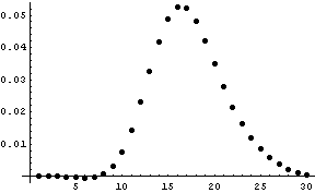
The maximum error is about 5%. It’s not an industrial quality random number generator, but it’s perfectly adequate for classroom demonstrations.

Now what would happen if we rolled more than five dice? We’d expect a better approximation. In fact, we can be more precise. The central limit theorem suggests that as we roll n dice, the maximum error will be proportionate to 1/√ n when n is large. So if we roll four times as many dice, we’d expect the error to go down by a factor of two. In fact, that’s just what we see. When we go from 5 dice to 20 dice, the maximum error goes from 0.0525 to 0.0262.

Three reasons expert predictions are often wrong

Posted on 9 February 2009 by John

A comment on Twitter this morning reminded me of a few points from Philip Tetlock’s book Expert Political Judgment.

Experts are under pressure to form opinions quickly so they can respond to interviewers.
You don’t get invited to appear on talk shows for having conventional opinions. An expert who, after long deliberation, decides things are going to continue the way they’ve been going is not likely to appear in the press. This causes a selection bias in the predictions that receive publicity. It also creates incentives for experts to make sensational predictions.
Experts have many facts to draw on, and so can be uncommonly good at confirming incorrect beliefs. Someone less knowledgeable might be forced to do some research.

Tetlock’s book focuses on political experts, though the same principles apply to other areas.

The smoothest curve through a set of points

Posted on 6 February 2009 by John

How do you fit the smoothest curve through a set of points? Suppose you have a set of increasing x values x₁, x₂, x₃, … , x_n and a corresponding set of y values y₁, y₂, y₃, … , y_n. You want to find the smoothest function f(x) such that f(x_i) = y_i for i = 1, 2, 3, …, n. The smoothest curve depends on how you define smoothness, but we’ll develop a common definition that leads to a nice solution.

Our definition of smoothness starts with the second derivative. If a curve is flat, it has zero second derivative. If the curve has a sharp kink, the second derivative will be high there. We want to add up the smoothness over the entire curve, so we’ll integrate the second derivative. But that won’t quite work. Second derivatives can be positive or negative, and a curve could have several sharp bends and still have average second derivative zero. Sharp bends in one direction could be canceled out by equally sharp bends in the opposite direction. So we look at the square of the second derivative. That gives a positive number whether the curve bends up or down. Also, squaring small numbers makes them smaller and squaring big numbers makes them bigger. So squaring the second derivative will penalize sharp bends and be more forgiving of small bends. In summary, we’ll measure the smoothness of a function f(x) over an interval [a, b] by the following integral.

$\int_a^b \left( f''(x) \right)^2\, dx$

Using the above measure of smoothness, the smoothest function interpolating a set of values is a natural cubic spline. I’ll explain this definition from right to left: first I’ll explain what a spline is, then a cubic spline, then a natural cubic spline. Cubic splines are very commonly used in graphical applications.

A spline is a function made by piecing together other functions. Most splines are piecewise polynomials, though there are other kinds of splines, such as trigonometric splines that are piecewise trig functions. The term “spline” comes from a mechanical device for drawing curves.

A cubic spline is formed by piecing together cubic polynomials. That is, the restriction of f to any interval between two x-values, from x_i to x_i+1 is a cubic polynomial. These piecewise cubic polynomials are formed by making their first and second derivatives match where they join. This makes a cubic spline curve appear very smooth.

Say we have n values of x and y. That means we have n-1 cubic polynomials to fit together: one over [x₁, x₂], another over [x₂, x₃], etc. Each cubic polynomial has 4 coefficients, and so we have a total of 4(n-1) coefficients to determine. At each interior node, i.e. the values from x₂ to x_n-1, there are four constraints. At each such x_i we have

The polynomial on the left side must have value y_i.
The polynomial on the right side must have value y_i.
The first derivatives of the left and right polynomials must match.
The second derivatives of the left and right polynomials must match.

This gives us a total of 4(n-2) interior constraints. The values at the left and right ends are specified too, i.e. f(x₁) = y₁ and f(x_n) = y_n. This adds up to 4n-6 constraints on 4n-4 coefficients. We need two more constraints to have as many equations as unknowns. There are various ways to add these constraints but a natural cubic spline imposes the requirement that the second derivatives should be zero at the ends, i.e. f”(x₁) = f”(x_n) = 0.

Finding the coefficients for a natural cubic spline with n nodes requires solving 4n – 4 equations in as many unknowns. There is a unique solution to this system of equations, and the system has a special structure that can be solved very quickly.

One thing I find interesting about natural cubic splines is how a fairly ad hoc procedure — patching cubic polynomials — leads to the solution to an elegant minimization problem.

Related: Help with interpolation

Example of SQL problem

Posted on 6 February 2009 by John

Here’s an excerpt from an email someone sent me in response to my post previous post Why SQL failed.

…

Your SQL blog article got my attention since I recently had to fix some SQL code that someone else wrote that has been in production for the last 4 years, running on a dataset containing about 3 million records. It performed some compound operations like the following.
SELECT *
FROM TESTTB2
WHERE
(COL1 IN (‘A', ‘B', ‘F')
AND
COL1 NOT IN (‘X','Y','Z')
OR
COL1 <> ‘R')
If the column COL1 contained null(s), then the NOT IN tests did not work as expected.

In the SQL code I was fixing, the SELECT missed 49,000 records that the programmer thought were being selected! The take-away message is that SQL requires attention to detail that often is not realized by the hobbyist programmer.

Programming

Statistics

Productivity / creativity

History