The other day I ran across a blog post by Brian Hayes that linked to an article by David Cantrell on how to compute the inverse of the gamma function. Cantrell gives an approximation in terms of the Lambert W function.
In this post we’ll write a little Python code to kick the tires on Cantrell’s approximation. The post also illustrates how to do some common tasks using SciPy and matplotlib.
Here are the imports we’ll need.
      import matplotlib.pyplot as plt
      from scipy import pi, e, sqrt, log, linspace
      from scipy.special import lambertw, gamma, psi
      from scipy.optimize import root
First of all, the gamma function has a local minimum k somewhere between 1 and 2, and so it only makes sense to speak of its inverse to the left or right of this point. Gamma is strictly increasing for real values larger than k.
To find k we look for where the derivative of gamma is zero. It’s more common to work with the derivative of the logarithm of the gamma function than the derivative of the gamma function itself. That works just as well because gamma has a minimum where its log has a minimum. The derivative of the log of the gamma function is called ψ and is implemented in SciPy as scipy.special.psi. We use the function scipy.optimize.root to find where ψ is zero.
The root function returns more information than just the root we’re after. The root(s) are returned in the arrayx, and in our case there’s only one root, so we take the first element of the array:
k = root(psi, 1.46).x[0]
Now here is Cantrell’s algorithm:
      c = sqrt(2*pi)/e - gamma(k)

      def L(x):
          return log((x+c)/sqrt(2*pi))

      def W(x):
          return lambertw(x)

      def AIG(x):
          return L(x) / W( L(x) / e) + 0.5
Cantrell uses AIG for Approximate Inverse Gamma.
How well goes this algorithm work? For starters, we’ll see how well it does when we do a round trip, following the exact gamma with the approximate inverse.
      x = linspace(5, 30, 100)
      plt.plot(x, AIG(gamma(x)))
      plt.show()
This produces the following plot:
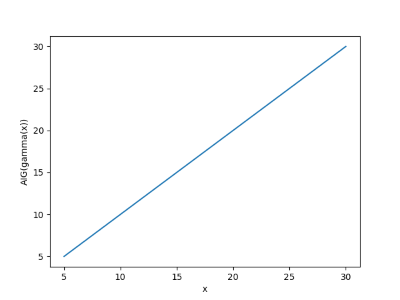
We get a straight line, as we should, so next we do a more demanding test. We’ll look at the absolute error in the approximate inverse. We’ll use a log scale on the x-axis since gamma values get large quickly.
      y = gamma(x)
      plt.plot(y, x- AIG(y))
      plt.xscale("log")
      plt.show()
This shows the approximation error is small, and gets smaller as its argument increases.
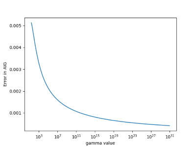
Cantrell’s algorithm is based on an asymptotic approximation, so it’s not surprising that it improves for large arguments.
Comments are closed.