The previous post looked at a particular cellular automaton, the so-called Rule 90. When started with a single pixel turned on, it draws a Sierpinski triangle. With random starting pixels, it draws a semi-random pattern that retains features like the Sierpinski triangle.
There are only 256 possible elementary cellular automata, so it’s practical to plot them all. I won’t list all the images here—you can find them all here—but I will give a few examples to show the variety of patterns they produce. As in the previous post, we imagine our grid rolled up into a cylinder, i.e. we’ll wrap around if necessary to find pixels diagonally up to the left and right.
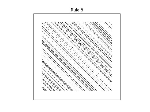
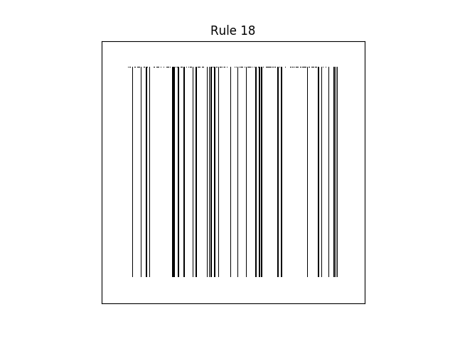
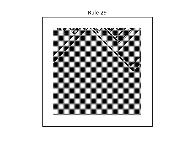
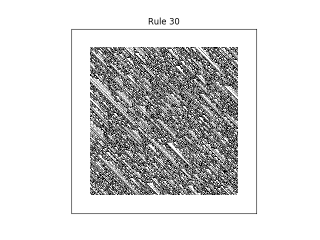
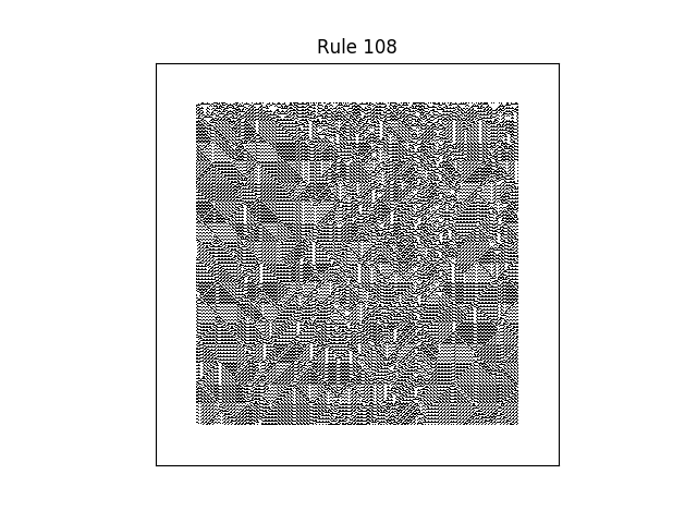
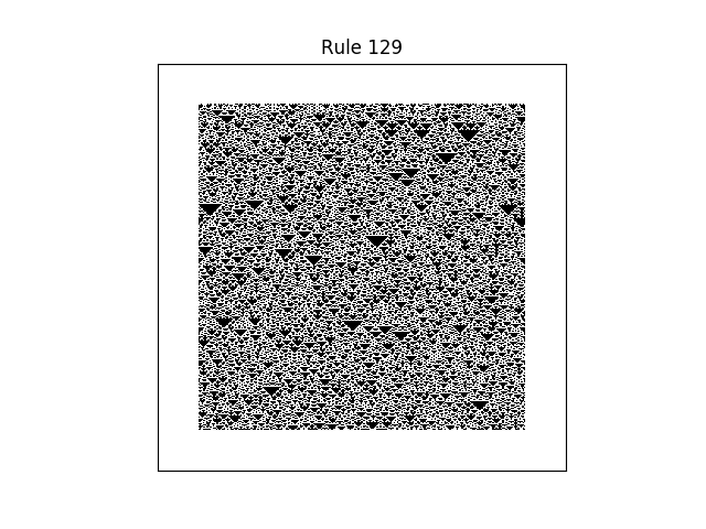
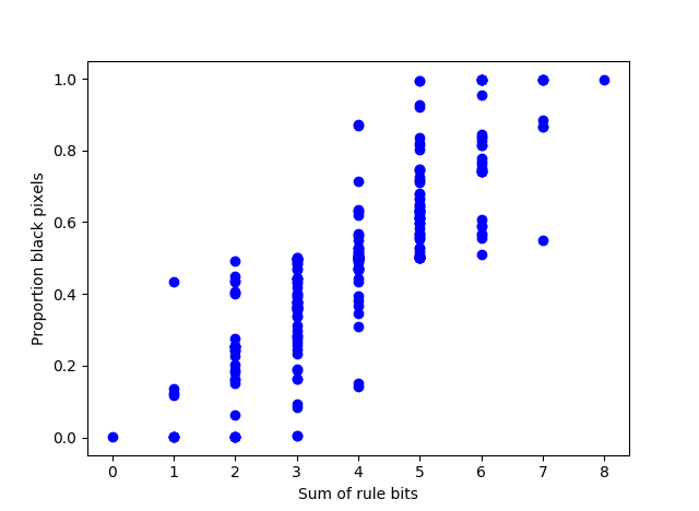
As we discussed in the previous post, the number of a rule comes from what value it assigns to each of eight possible cellular states, turned into a binary number. So it’s plausible that binary numbers with more 1’s correspond to more black pixels. This is roughly true, though the graph below shows that the situation is more complex than that.
Is the composition of two simple automata a simple automata?
You run one pass with an automaton, and one pass with another. And so forth.
Daniel: With two steps, you depend on a context of five cells instead of three.
@daniel:
Only the first row (initial conditions) matters since the second pass would overwrite everything after the first row
The proportion of black pixels graph is antisymmetric – cool!
But when you think about it, the way one’s and zero’s are used here is symmetric – you could have used zero’s and one’s and inverted the output for the same results