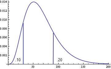
The doctor says 10% of patients respond within 30 days of treatment and 80% respond within 90 days of treatment. Now go turn that into a probability distribution. That’s a common task in Bayesian statistics, capturing expert opinion in a mathematical form to create a prior distribution.

Things would be easier if you could ask subject matter experts to express their opinions in statistical terms. You could ask “If you were to represent your belief as a gamma distribution, what would the shape and scale parameters be?” But that’s ridiculous. Even if they understood the question, it’s unlikely they’d give an accurate answer. It’s easier to think in terms of percentiles.

Asking for mean and variance are not much better than asking for shape and scale, especially for a non-symmetric distribution such as a survival curve. Anyone who knows what variance is probably thinks about it in terms of a normal distribution. Asking for mean and variance encourages someone to think about a symmetric distribution.

So once you have specified a couple percentiles, such as the example this post started with, can you find parameters that meet these requirements? If you can’t meet both requirements, how close can you come to satisfying them? Does it depend on how far apart the percentiles are? The answers to these questions depend on the distribution family. Obviously you can’t satisfy two requirements with a one-parameter distribution in general. If you have two requirements and two parameters, at least it’s feasible that both can be satisfied.

If you have a random variable X whose distribution depends on two parameters, when can you find parameter values so that Prob(X ≤ x₁) = p₁ and Prob(X ≤ x₂) = p₂? For starters, if x₁ is less than x₂ then p₁ must be less than p₂. For example, the probability of a variable being less than 5 cannot be bigger than the probability of being less than 6. For some common distributions, the only requirement is this requirement that the x‘s and p‘s be in a consistent order.

For a location-scale family, such as the normal or Cauchy distributions, you can always find a location and scale parameter to satisfy two percentile conditions. In fact, there’s a simple expression for the parameters. The location parameter is given by

and the scale parameter is given by

where F(x) is the CDF of the distribution representative with location 0 and scale 1.

The shape and scale parameters of a Weibull distribution can also be found in closed form. For a gamma distribution, parameters to satisfy the percentile requirements always exist. The parameters are easy to determine numerically but there is no simple expression for them.

For more details, see Determining distribution parameters from quantiles. See also the ParameterSolver software.

Update: I posted an article on CodeProject with Python code for computing the parameters described here.

Related posts

• Biostatistics software
• Diagram of distribution relationships
• How to calculate percentiles in memory-bound applications
• Consulting in Bayesian analysis

Here’s another quote from Anthony O’Hagan’s book Bayesian Inference.

All classical inference statements … are probability statements about x given θ, phrased so as to appear to be probability statements about θ.

Emphasis in the original.

More statistical posts

• Four reasons to use Bayesian inference
• Four pillars of Bayesian statistics

The following is a direct quote from Anthony O’Hagan’s book Bayesian Inference. I’ve edited the quote only to enumerate the points.

Why should one use Bayesian inference, as opposed to classical inference? There are various answers. Broadly speaking, some of the arguments in favour of the Bayesian approach are that it is

1. fundamentally sound,
2. very flexible,
3. produces clear and direct inferences,
4. makes use of all available information.

I’ll elaborate briefly on each of O’Hagan’s points.

Bayesian inference has a solid philosophical foundation. It is consistent with certain axioms of rational inference. Non-Bayesian systems of inference, such as fuzzy logic, must violate one or more of these axioms; their conclusions are rationally satisfying to the extent that they approximate Bayesian inference.

Bayesian inference is at the same time rigid and flexible. It is rigid in the sense that all inference follows the same form: set up a likelihood and a prior, then calculate the posterior by conditioning on observed data via Bayes theorem. But this rigidity channels creativity into useful directions. It provides a template for setting up complex models when necessary.

Frequentist inferences are awkward to explain. For example, confidence intervals and p-values are tedious to define rigorously. Most consumers of confidence intervals and p-values do not know what they mean and implicitly assume Bayesian interpretations. The difference is not simply pedantic. Particularly with regard to p-values, the common understanding can be grossly inaccurate. By contrast, Bayesian counterparts are simple to define and interpret. Bayesian credible intervals are exactly what most people think confidence intervals are. And a Bayesian hypotheses test simply compares the probability of each hypothesis via Bayes factors.

Sometimes the necessity of specifying prior distributions is seen as a drawback to Bayesian inference. On the other hand, the ability to specify prior distributions means that more information can be incorporated in an inference. See Musicians, drunks, and Oliver Cromwell for a colorful illustration from Jim Berger on the need to incorporate prior information.

More posts on Bayesian statistics

• Four pillars of Bayesian statistics
• Bayesian statistics is misnamed
• What is a confidence interval?

I’m teaching an introduction to Bayesian statistics. My first thought was to start with Bayes theorem, as many introductions do. But this isn’t the right starting point. Bayes’ theorem is an indispensable tool for Bayesian statistics, but it is not the foundational principle. The foundational principle of Bayesian statistics is the decision to represent uncertainty by probabilities. Unknown parameters have probability distributions that represent the uncertainty in our knowledge of their values.

Once you decide to use probabilities to express parameter uncertainty, you inevitably run into the need for Bayes theorem to work with these probabilities. Bayes theorem is applied constantly in Bayesian statistics, and that is why the field takes its name from the theorem’s author, Reverend Thomas Bayes (1702-1761). But “Bayesian” doesn’t describe Bayesian statistics quite the same way that “Frequentist” described frequentist statistics. The term “frequentist” gets to the heart of how frequentist statistics interprets probability. But “Bayesian” refers to a Bayes theorem, a computational tool for carrying out probability calculations in Bayesian statistics. If frequentist statistics were analogously named, it might be called “Bernoullian statistics” after Jacob Bernoulli’s law of large numbers.

The term “Bayesian” statistics might imply that frequentist statisticians dispute Bayes’ theorem. That is not the case. Bayes’ theorem is a simple mathematical result. What people dispute is the interpretation of the probabilities that Bayesians want to stick into Bayes’ theorem.

I don’t have a better name for Bayesian statistics. Even if I did, the name “Bayesian” is firmly established. It’s certainly easier to say “Bayesian statistics” than to say “that school of statistics that represents uncertainty in unknown parameters by probabilities,” even though the latter is accurate.

More Bayesian posts

• Four pillars of Bayesian statistics
• What a probability means
• The probability that Shakespeare wrote a play

Anthony O’Hagan’s book Bayesian Inference lists four basic principles of Bayesian statistics at the end of the first chapter:

1. Prior information. Bayesian statistics provides a systematic way to incorporate what is known about parameters before an experiment is conducted. As a colleague of mine says, if you’re going to measure the distance to the moon, you know not to pick up a yard stick. You always know something before you do an experiment.
2. Subjective probability. Some Bayesians don’t agree with the subjective probability interpretation, but most do, in practice if not in theory. If you write down reasonable axioms for quantifying degrees of belief, you inevitably end up with Bayesian statistics.
3. Self-consistency. Even critics of Bayesian statistics acknowledge that Bayesian statistics has a rigorous self-consistent foundation. As O’Hagan says in his book, the difficulties with Bayesian statistics are practical, not foundational, and the practical difficulties are being resolved.
4. No adhockery. Bruno de Finetti coined the term “adhockery” to describe the profusion of frequentist methods. More on this below.

This year I’ve had the chance to teach a mathematical statistics class primarily focusing on frequentist methods. Teaching frequentist statistics has increased my appreciation for Bayesian statistics. In particular, I better understand the criticism of frequentist adhockery.

For example, consider point estimation. Frequentist statistics to some extent has standardized on minimum variance unbiased estimators as the gold standard. But why? And what do you do when such estimators don’t exist?

Why focus on unbiased estimators? Granted, lack of bias sounds like a good thing to have. All things being equal, it would be better to be unbiased than biased. But all things are not equal. Sometimes unbiased estimators are ridiculous. Why only consider biased vs. unbiased rather, a binary choice, rather than degree of bias, a continuous choice? Efficiency is also important, and someone may reasonably accept a small amount of bias in exchange for a large increase in efficiency.

Why minimize expected mean squared error? Efficiency in classical statistics is typically measured by expected mean squared error. But why not minimize some other measure of error? Why use an exponent of 2 and not 1, or 4, or 2.738? Or why limit yourself to power functions at all? The theory is simplest for squared error, and while this is a reasonable choice in many applications, it is still an arbitrary choice.

How much emphasis should be given to robustness? Once you consider robustness, there are infinitely many ways to compromise between efficiency and robustness.

Many frequentists are asking the same questions and are investigating alternatives. But I believe these alternatives are exactly what de Finetti had in mind: there are an infinite number of ad hoc choices you can make. Bayesian methods are criticized because prior distributions are explicitly subjective. But there are myriad subjective choices that go into frequentist statistics as well, though these choices are often implicit.

There is a great deal of latitude in Bayesian statistics as well, but the latitude is confined to fit within a universal framework: specify a likelihood and prior distribution, then update the model with data to compute the posterior distribution. There are many ways to construct a likelihood (exactly as in frequentist statistics), many ways to specify a prior, and many ways to summarize the information contained in the posterior distribution. But the basic framework is fixed. (In fact, the framework is inevitable given certain common-sense rules of inference.)

More statistical posts

• Probability and information
• What is a confidence interval?