The Smith chart from electrical engineering is the image of a Cartesian grid under the function
f(z) = (z − 1)/(z + 1).
More specifically, it’s the image of a grid in the right half-plane.
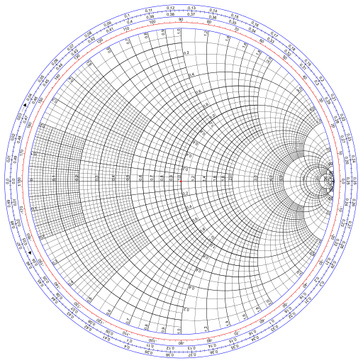
This post will derive the basic mathematical properties of this graph but will not go into the applications. Said another way, I’ll explain how to make a Smith chart, not how to use one.
We will use z to denote points in the right half-plane and w to denote the image of these points under f. We will speak of lines in the z plane and the circles they correspond to in the w plane.
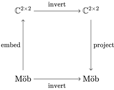
Möbius transformations
Our function f is a special case of a Möbius transformation. There is a theorem that says Möbius transformation map generalized circles to generalized circles. Here a generalized circle means a circle or a line; you can think of a line as a circle with infinite radius. We’re going to get a lot of mileage out of that theorem.
Image of the imaginary axis
The function f maps the imaginary axis in the z plane to the unit circle in the w plane. We can prove this using the theorem above. The imaginary axis is a line, so it’s image is either a line or a circle. We can take three points on the imaginary axis in the z plane and see where they go.
When we pick z equal to 0, i, and −i from the imaginary axis we get w values of −1, i, and −i. These three w values do not line on a line, so the image of the imaginary axis must be a circle. Furthermore, three points uniquely determine a circle, so the image of the imaginary axis is the circle containing −1, i, and −i, i.e. the unit circle.
Image of the right half-plane
The imaginary axis is the boundary of the right half-plane. Since it is mapped to the unit circle, the right half-plane is either mapped to the interior of the unit circle or the exterior of the unit circle. The point z = 1 goes to w = 0, and so the right half-plane is mapped inside the unit circle.
Images of vertical lines
Let’s think about what happens to vertical lines in the z plane, lines with constant positive real part. The images of these lines in the w plane must be either lines or circles. And since the right-half plane gets mapped inside the unit circle, these lines must get mapped to circles.
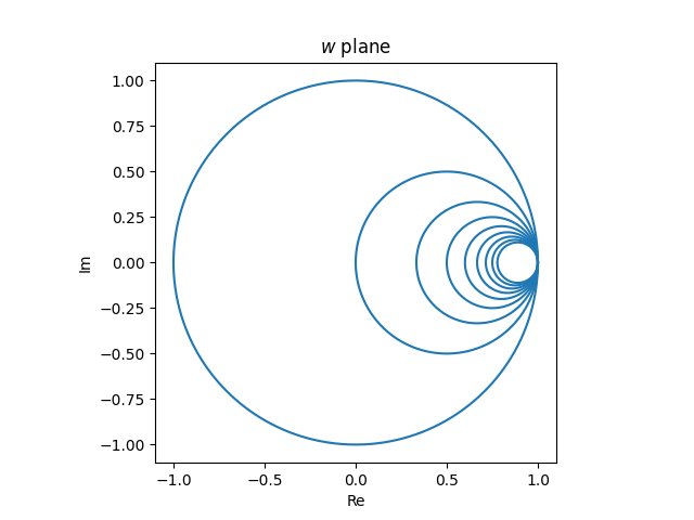
We can say a little more. All lines contain the point ∞, and f(∞) = 1, so the image of every vertical line in the z plane is a circle in the w plane, inside the unit circle and tangent to the unit circle at w = 1. (Tossing around ∞ is a bit informal, but it’s easy to make rigorous.)
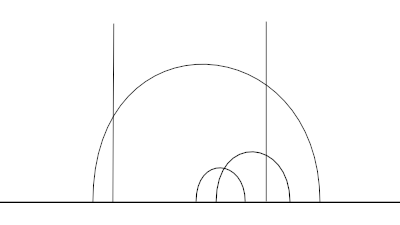
The vertical lines in the z plane
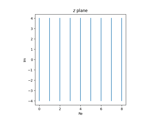
map to tangent circles in the w plane.
Images of horizontal lines
Next, let’s think about horizontal lines in the z plane, lines with constant imaginary part. The image of these lines is either a line or a circle. Which is it? The image of a line is a line if it contains ∞, otherwise it’s a circle. Now f(z) = ∞ if and only if z = −1, and so the image of the real axis is a line, but the image of every other horizontal line is a circle.
Since f(∞) = 1, the image of every horizontal line passes through 1, just as the images of all the vertical lines passes through 1.
Since horizontal lines extend past the right half-plane, the image circles extend past the unit circle. The part of the line with positive real part gets mapped inside the unit circle, and the part of the line with negative real part gets mapped outside the unit circle. In particular, the image of the positive real axis is the interval [−1, 1].
Möbius transformations are conformal maps, and so they preserve angles of intersection. Since horizontal lines are perpendicular to vertical lines, the circles that are the images of the horizontal lines meet the circles that are the images of vertical lines at right angles.
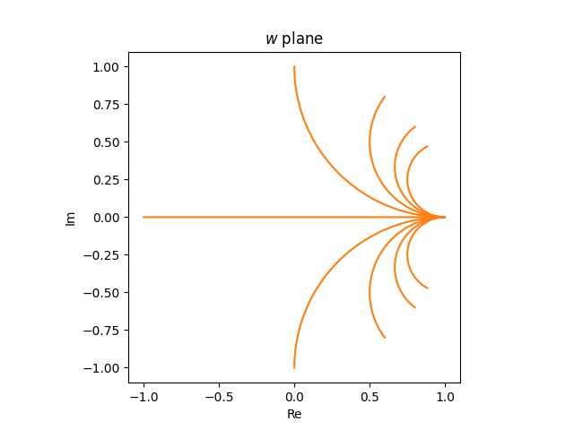
The horizontal rays in the z plane
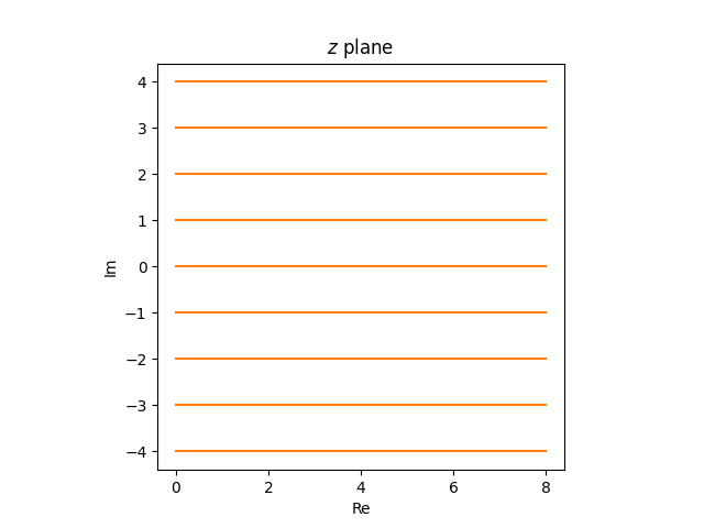
become partial circles in the w plane.
If we were to look at horizontal lines rather than rays, i.e. if we extended the lines into the left half-plane, the images in the w plane would be full circles.
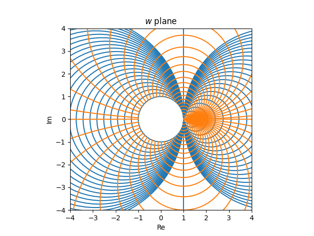
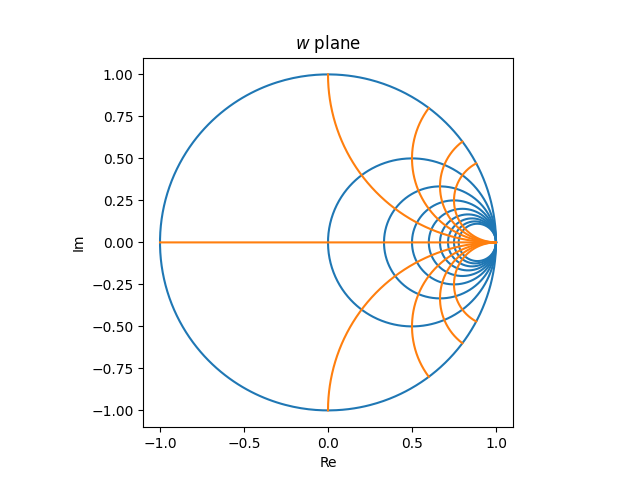
Now let’s put our images together. The grid
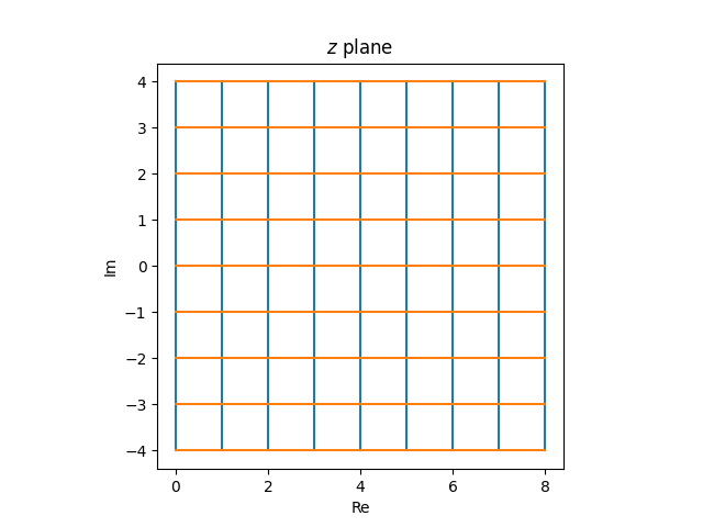
in the z plane becomes the following in the w plane.
Spacing
An evenly spaced grid in the z plane becomes a very unevenly spaced graph in the w plane. Things are crowded on the right hand side and sparse on the left. A usable Smith chart needs to be roughly evenly filled in, which means it has to be the image of an unevenly filled in grid in the z plane. For example, you’d need more vertical lines in the z plane with small real values than with large real values.
I address the issue of spacing in the next post.