Atonal music is difficult to compose because it defies human instincts. It takes discipline to write something so unpleasant to listen to.
One technique that composers use to keep their music from falling into tonal patterns is the twelve-tone row. The composer creates some permutation of the 12 notes in a chromatic scale and then uses these notes strictly in order. The durations of the notes may vary, and the notes may move up or down octaves, but the pitch classes are recycled over and over in order.
There are variations on this technique that allow a small amount of variety, such as allowing the the tone row to be reversed, inverted, or both. The retrograde version of the sequence is the original (prime) sequence of notes in the opposite order. The inverted form of the tone row inverts each of the intervals in the original sequence, going up by k half steps when the original when down by k half steps and vice versa. The retrograde inverted sequence is the inverted sequence in the opposite order.
Here is an example, taken from Arnold Schoenberg’s Suite for Piano, Op. 25.

Some math
Since a tone row is a permutation of 12 notes, there are 12! possible tone rows. However, since the notes of a tone row are played in a cycle, the same sequence of notes starting at a different point shouldn’t count as a distinct tone row. With that way of counting, there are 11! possible tone rows.
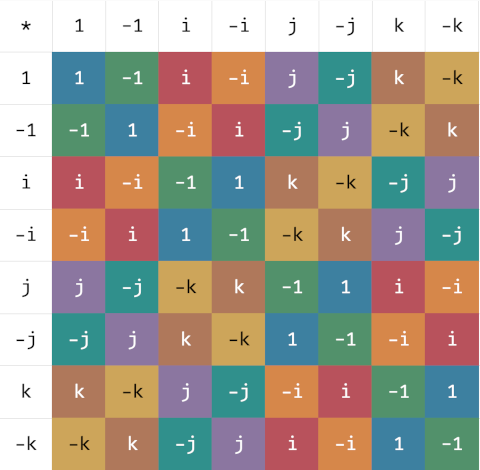
The operations of creating the retrograde and inverted forms of a tone row are the generators of an Abelian group. Let P (for prime) be the null operation, leaving a sequence alone. Then the elements of the group are P, R, I, and RI (= IR). The two generators have order 2, i.e. R² = I² = P. Therefore the group is isomorphic to ℤ2 × ℤ2.
Although I enjoy music and math, I do not enjoy most attempts to use math to compose music. I do not like atonal music, though I do like some “math rock.” It seems that math applied to rhythm results in more palatable music than math applied to melody.
Update: More math in the next post. Do the applications of R, I, and RI always produce different sequences of notes? What if you consider two rotations of a tone row to be equivalent?
A concert story
When I was in college I often walked from my dorm over the music building for concerts. I probably heard more concerts in college than I have heard ever since.
One night I went to an organ concert. At the end of the concert the organist took melodies on strips of paper that he had not seen before and improvised a fugue on each. After the concert I ran into a friend in the music building who had not been to the concert. I enthusiastically told him how impressed I was by the improvised fugues, especially the last one that sounded like Schoenberg tone row.
The organist overhead my conversation and walked up to me and said that he was impressed that I recognized the Schoenberg tone row. To be fair, I did not recognize the music per se. The music sounded random, and I came up with the only example of random music I could think of, and said it sounded like a Schoenberg tone row. I certainly did not say “Ah, yes. That was Schoenberg’s tone row from ….” It was a lucky guess.