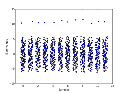
Mark Kac asked in 1966 whether you can hear the shape of a drum. In other words, can two drums, made of the same material, produce the exact same sound but have different shapes? More formally, Kac asked whether the eigenvalues of the Laplace’s equation with zero boundary conditions uniquely determine the shape of a region in the plane. The question remained open until 1992. No, you can’t always hear the shape of a drum. But often you can. With some restrictions on the regions, the shape is uniquely determined by the sound, i.e., the Laplace spectrum.
Ten years before Kac asked about hearing the shape of a drum, Günthard and Primas asked the analogous question about graphs. Can you hear the shape of a graph? That is, can two different graphs have the same eigenvalues? At the time, the answer was believed to be yes, but a year later it was found to be no, not always [1]. So the next natural question is when can you hear the shape of a graph, i.e. under what conditions is a graph determined by its eigenvalues? It depends on which matrix you’re taking the eigenvalues of, but under some conditions some matrix spectra uniquely determine graphs. We don’t know in general how common it is for spectra to uniquely determine graphs.
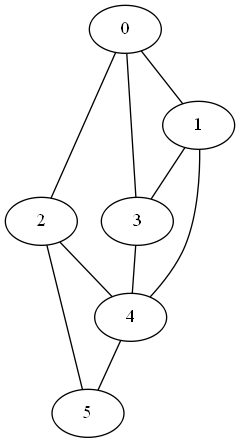
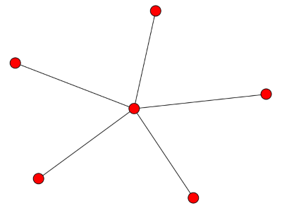
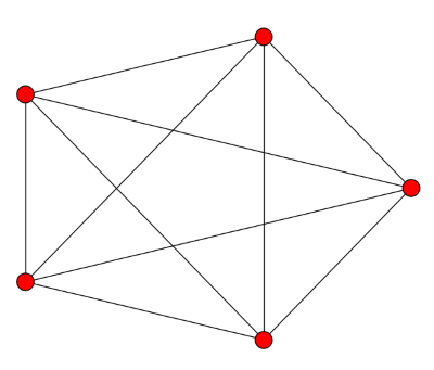
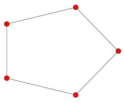
Here are two graphs that have the same adjacency matrix spectra, first published in [2]:
Both have adjacency spectra [-2, 0, 0, 0, 2]. But the graphs are not cospectral as far as the Laplacian is concerned. Their Laplace spectra are [0, 0, 2, 2, 4] and [0, 1, 1, 1, 5] respectively. We could tell that the Laplace spectra would be different before computing them because the second smallest Laplace eigenvalue is positive if and only if a graph is connected.
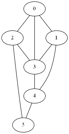
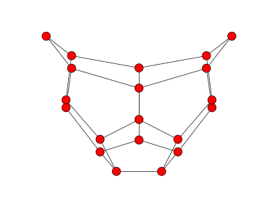
The graphs below are cospectral for the adjacency, Laplacian, and unsigned Laplacian matrices.
Both graphs have the same number of nodes and edges, and every node has degree 4 in both graphs. But the graph on the left contains more triangles than the one on the right, so they cannot be isomorphic.
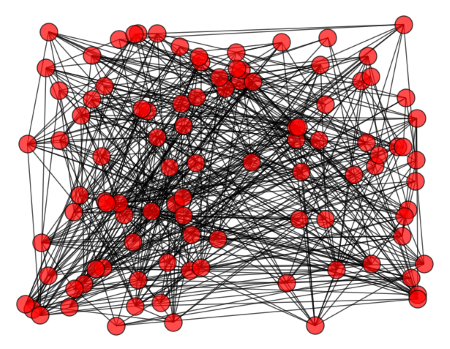
One way to test whether two graphs are isomorphic is to compute their spectra. If the spectra are different, the graphs are not isomorphic. So spectral analysis gives a way to show that two graphs are not isomorphic in polynomial time, though the test may be inconclusive.
If two graphs do have the same spectra, what is the probability that they are isomorphic? In [1] the authors answer this question empirically for graphs of order up to 11. Very roughly, there’s about an 80% chance graphs with the same adjacency matrix spectrum are isomorphic. The chances go up to 90% for the Laplacian and 95% for the signless Laplacian.
***
[1] Edwin R. van Dam, Willem H. Haemers. Which graphs are determined by their spectrum? Linear Algebra and its Applications 373 (2003) 241–272
[2] D.M. Cvetkovi´c, Graphs and their spectra, Univ. Beograd. Publ. Elektrotehn. Fak. Ser. Mat. Fiz. 354–356 (1971) 1–50.


![\left[ \begin{array}{rrrrr} 4 & -1 & -1 & -1 & -1 \\ -1 & 4 & -1 & -1 & -1 \\ -1 & -1 & 4 & -1 & -1 \\ -1 & -1 & -1 & 4 & -1 \\ -1 & -1 & -1 & -1 & 4 \end{array} \right]](http://www.johndcook.com/complete_graph_laplacian.png)
![\left[ \begin{array}{cccccc} 5 & -1 & -1 & -1 & -1 & -1 \\ -1 & 1 & 0 & 0 & 0 & 0 \\ -1 & 0 & 1 & 0 & 0 & 0 \\ -1 & 0 & 0 & 1 & 0 & 0 \\ -1 & 0 & 0 & 0 & 1 & 0 \\ -1 & 0 & 0 & 0 & 0 & 1 \end{array} \right]](http://www.johndcook.com/star_graph_laplacian.png)
![\left[ \begin{array}{rrrrr} 2 & -1 & 0 & 0 & -1 \\ -1 & 2 & -1 & 0 & 0 \\ 0 & -1 & 2 & -1 & 0 \\ 0 & 0 & -1 & 2 & -1 \\ -1 & 0 & 0 & -1 & 2 \\ \end{array} \right]](http://www.johndcook.com/cycle_graph_laplacian.png)