Cover time of a graph: cliques, chains, and lollipops

Posted on 4 January 2017 by John

Cover time

The cover time of a graph is the expected time it takes a simple random walk on the graph to visit every node. A simple random walk starts at some node, then at each step chooses with equal probability one of the adjacent nodes. The cover time is defined to be the maximum over all starting points of expected time to visit all nodes.

It seems plausible that adding edges to a graph would decrease its cover time. Sometimes this is the case and sometimes it isn’t, as we’ll demonstrate below.

Chains, complete graphs, and lollipops

This post will look at three kinds of graphs

a chain of n vertices
a complete graph on n vertices
a “lollipop” with n vertices

A chain simply connects vertices in a straight line. A complete graph connects every node to every other node.

A lollipop graph of order (5, 5)

A lollipop with n vertices takes a chain with n/2 vertices and complete graph on n/2 vertices and joins them together. The image above is a lollipop graph of order 10. The complete graph becomes a clique in the new graph.

The image looks more like a kite than a lollipop because that’s the way my software (networkx) drew it by default. If you’d like, image the complete graph more round and the chain more straight so that the graph more closely resembles a lollipop.

Random walks on graphs

Chains have a long cover time. Complete graphs have a short cover time. What about lollipops?

A plausible answer would be that a lollipop graph would have a moderate cover time, somewhere between that of a complete graph and a chain. But that’s not the case. In fact, the lollipop has a longer cover time than either the complete graph or the chain.

You could think of a lollipop graph with n vertices as a chain of length n with extra edges added. This shows that adding edges does not always decrease the cover time.

The cover times for the three graphs we consider here are of different orders: O(n log n) for the complete graph, O(n²) for the chain, and O(n³) for the lollipop.

Now these are only asymptotic results. Big-O notation leaves out proportionality constants. We know that for sufficiently large n the cover times are ordered so that the complete graph is the smallest, then the chain, then the lollipop. But does n have to be astronomically large before this happens? What happens with a modest size n?

There’s a theoretical result that says the cover time is bounded by 2m(n-1) where m is the number of edges and n the number of vertices. This tells us that when we say the cover time for the chain is O(n²) we can say more, that it’s less than 2n², so at least in this case the proportionality constant isn’t large.

We’ll look at the cover times with some simulation results below based on n = 10 and n = 30 based on 10,000 runs.

With 10 nodes each, the cover times for the complete graph, chain, and lollipop were 23.30, 82.25, and 131.08 respectively.

With 30 nodes the corresponding cover times were 114.37, 845.16, and 3480.95.

So the run times were ordered as the asymptotic theory would suggest.

Rapidly mixing random walks on graphs

Posted on 24 December 2016 by John

Random walks mix faster on some graphs than on others. Rapid mixing is one of the ways to characterize expander graphs.

By rapid mixing we mean that a random walk approaches its limiting (stationary) probability distribution quickly relative to random walks on other graphs.

Here’s a graph that supports rapid mixing. Pick a prime p and label nodes 0, 1, 2, 3, …, p-1. Create a circular graph by connecting each node k to k+1 (mod p). Then add an edge between each non-zero k to its multiplicative inverse (mod p). If an element is its own inverse, add a loop connecting the node to itself. For the purpose of this construction, consider 0 to be its own inverse. This construction comes from [1].

Here’s what the graph looks like with p = 23.

Cayley graph of order 23

This graph doesn’t show the three loops from a node to itself, nodes 1, 0, and 22.

At each node in the random walk, we choose an edge uniformly and follow it. The stationary distribution for a random walk on this graph is uniform. That is, in the long run, you’re equally likely to be at any particular node.

If we pick an arbitrary starting node, 13, and take 30 steps of the random walk, the simulated probability distribution is nearly flat.

By contrast, we take a variation on the random walk above. From each node, we move left, right, or stay in place with equal probability. This walk is not as well mixed after 100 steps as the original walk is after only 30 steps.

You can tell from the graph that the walk started around 13. In the previous graph, evidence of the starting point had vanished.

The code below was used to produce these graphs.

To investigate how quickly a walk on this graph converges to its limiting distribution, we could run code like the following.

    from random import random
    import numpy as np
    import matplotlib.pyplot as plt
    m = 23

    # Multiplicative inverses mod 23
    inverse = [0, 1, 12, 8, 6, 14, 4, 10, 3, 18, 7, 21, 2, 16, 5, 20, 13, 19, 9, 17, 15, 11, 22]

    # Verify that the inverses are correct
    assert(len(inverse) == m)
    for i in range(1, m):
        assert (i*inverse[i] % 23 == 1)

    # Simulation
    num_reps = 100000
    num_steps = 30

    def take_cayley_step(loc):
        u = random() * 3
        if u < 1: # move left
            newloc = (loc + m - 1) % m
        elif u < 2: # move right
            newloc = (loc + 1) % m
        else:
            newloc = inverse[loc] # or newloc = loc
        return newloc

    stats = [0]*m
    for i in range(num_reps):
        loc = 13 # arbitrary fixed starting point
        for j in range(num_steps):
            loc = take_cayley_step(loc)
        stats[loc] += 1

    normed = np.array(stats)/num_reps
    plt.plot(normed)
    plt.xlim(1, m)
    plt.ylim(0,2/m)
    plt.show()

* * *

[1] Shlomo Hoory, Nathan Linial, Avi Wigderson. “Expander graphs and their applications.” Bulletin of the American Mathematical Society, Volume 43, Number 4, October 2006, pages 439–561.

Ten spectral graph theory posts

Posted on 5 June 2016 by John

Erdős-Rényi graph

Here are 10 blog posts I wrote earlier this year about spectral graph theory, studying graphs via the eigenvalues of matrices associated with the graphs.

Personal growth and discrete harmonic functions

Posted on 9 April 2016 by John

“You are the average of the five people you spend the most time with.”

A Google search says this quote is by Jim Rohn. I think other people have said similar things. I’ve heard it quoted many times. The implication is usually that you can improve your life by hanging around better people.

Here are three things it makes me think of.

It sounds approximately true.
It can’t be literally true.
It reminds me of harmonic functions.

There are numbers to back up the assertion that things like your income and even your weight approximately match the average of the people around you. Cause and effect go both ways: people like to hang out with people like themselves, and we become like the people we hang around.

It’s an aphorism, not meant to be taken literally. But a moment’s thought shows that it can’t be literally true for everybody. In any social network, someone has the most money, for example. That person’s net worth cannot be the average of the net worth of others in the group, unless everyone has the exact same net worth. The same applies to the poorest person in the network.

The reason I say that this reminds me of harmonic functions is the mean value theorem. If a function satisfies Laplace’s equation in some region, at any point in the interior of the region, the value of the function equals the average of the function over a spherical region centered at the point. But this is only true in the interior. On the boundary, you might have a maximum or minimum. If the boundary is compact, you will have a maximum and a minimum, provided the function extends continuously to its boundary.

I think of the continuous case first because I spent years thinking about such things. But there’s a discrete analog of harmonic functions that applies directly to the example above. If you have some network, such as a social network, and assign number to each node, you have a discrete harmonic function if the value at every node is the average of the values at its neighboring nodes. For a finite network, a function cannot be harmonic at every point unless it is constant, for reasons given above. But a function could be harmonic at all but two nodes of a graph, or approximately harmonic at all nodes.

Graphs and square roots modulo a prime

Posted on 23 February 2016 by John

Imagine a clock with a prime number of hours. So instead of being divided into 12 hours, it might be divided into 11 or 13, for example. You can add numbers on this clock the way you’d add numbers on an ordinary clock: add the two numbers as ordinary integers and take the remainder by p, the number of hours on the clock. You can multiply them the same way: multiply as ordinary integers, then take the remainder by p. This is called arithmetic modulo p, or just mod p.

Which numbers have square roots mod p? That is, for which numbers x does there exist a number y such that y² = x mod p? It turns out that of the non-zero numbers, half have a square root and half don’t. The numbers that have square roots are called quadratic residues and the ones that do not have square roots are called quadratic nonresidues. Zero is usually left out of the conversation. For example, if you square the numbers 1 through 6 and take the remainder mod 7, you get 1, 4, 2, 2, 4, and 1. So mod 7 the quadratic residues are 1, 2, and 4, and the nonresidues are 3, 5, and 6.

A simple, brute force way to tell whether a number is a quadratic residue mod p is to square all the numbers from 1 to p-1 and see if any of the results equals your number. There are more efficient algorithms, but this is the easiest to understand.

At first it seems that the quadratic residues and nonresidues are scattered randomly. For example, here are the quadratic residues mod 23:

[1, 2, 3, 4, 6, 8, 9, 12, 13, 16, 18]

But there are patterns, such as the famous quadratic reciprocity theorem. We can see some pattern in the residues by visualizing them on a graph. We make the numbers mod p vertices of a graph, and join two vertices a and b with an edge if a–b is a quadratic residue mod p.

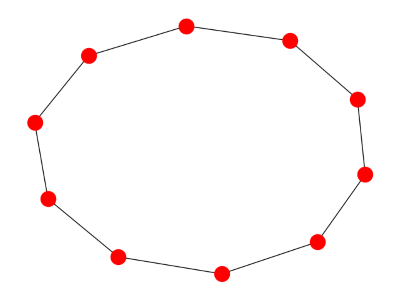
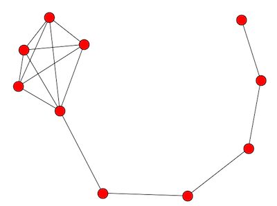
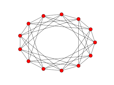
Here’s the resulting graph mod 13:

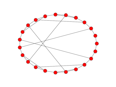
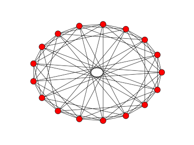
And here’s the corresponding graph for p = 17:

And here’s Python code to produce these graphs:

import networkx as nx
import matplotlib.pyplot as plt

def residue(x, p):
    for i in range(1, p):
        if (i*i - x) % p == 0:
            return True
    return False

p = 17
G = nx.Graph()
for i in range(p):
    for j in range(i+1, p):
        if residue(i-j, p):
            G.add_edge(i, j)

nx.draw_circular(G)
plt.show()

However, this isn’t the appropriate graph for all values of p. The graphs above are undirected graphs. We’ve implicitly assumed that if there’s an edge between a and b then there should be an edge between b and a. And that’s true for p = 13 or 17, but not, for example, for p = 11. Why’s that?

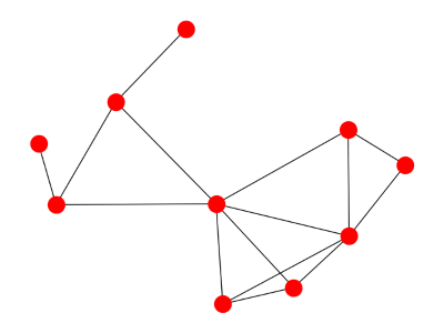
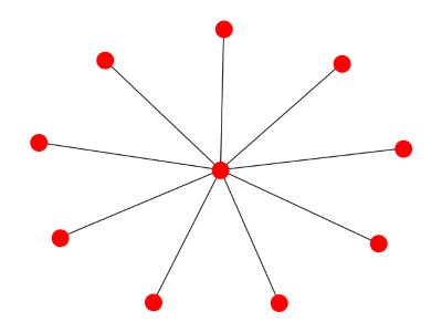
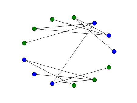
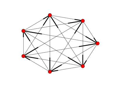
If p leaves a remainder of 1 when divided by 4, i.e. p = 1 mod 4, then x is a quadratic residue mod p if and only if –x is a quadratic residue mod p. So if a–b is a residue, so is b–a. This means an undirected graph is appropriate. But if p = 3 mod 4, x is a residue mod p if and only if –x is a non-residue mod p. This means we should use directed graphs if p = 3 mod 4. Here’s an example for p = 7.

The code for creating the directed graphs is a little different:

G = nx.DiGraph()
for i in range(p):
    for j in range(p):
        if residue(i-j, p):
            G.add_edge(i, j)

Unfortunately, the way NetworkX draws directed graphs is disappointing. A directed edge from a to b is drawn with a heavy line segment on the b end. Any suggestions for a Python package that draws more attractive directed graphs?

The idea of creating graphs this way came from Roger Cook’s chapter on number theory applications in Graph Connections. (I’m not related to Roger Cook as far as I know.)

You could look at quadratic residues modulo composite numbers too. And I imagine you could also make some interesting graphs using Legendre symbols.

Fourier transform of a function on a graph

Posted on 9 February 2016 by John

What is a Fourier transform at its core? An expansion of function in terms of eigenfunctions of the Laplacian. For a function on the real line, the Laplacian is simply the second derivative. The functions mapped to multiples of themselves by taking second derivatives are sines and cosines of various frequencies. A Fourier series is a change of basis, using as basis vectors those functions who behave the simplest under the second derivative.

The Fourier transform of a function on a graph is also a change of basis, expanding a discrete function in terms of eigenvalues of the Laplacian, in this case the graph Laplacian.

The Fourier transform of a function f, evaluated at a frequency ω, is the inner product of f with the eigenfunction exp(2πiωt).

$\hat{f}(\omega) = \langle f, \exp(2\pi i \omega t) \rangle = \int_{-\infty}^\infty f(t) \exp(-2\pi i \omega t) \, dx$

The inner product of two complex functions f and g is the integral of the product of f and the conjugate of g. Conjugation is why exp(2πiωt) became exp(-2πiωt).

The Fourier transform of a discrete function f on a graph, evaluated at an eigenvalue λ_i, is the inner product of f (i.e. the vector of values of f at each node) with the eigenvector associated with λ_i.

$\hat{f}(\lambda_i) = \langle f, v^*_i \rangle = \sum_{j=1}^N f(j) v_i^*(j)$

Here the inner product is a discrete sum rather than an integral. As before, we take the complex conjugate of the second item in the product.

The eigenvectors associated with the smallest eigenvalues of the graph Laplacian are analogous to low frequency sines and cosines. The eigenvalue components corresponding to nearly vertices in a graph should be close together. This analogy explains why spectral coordinates work so well.

Discrete harmonic functions

Posted on 4 February 2016 by John

A (continuous) harmonic function f on an open set a function that is twice differentiable and satisfied Laplace’s equation: ∇² f = 0. Such functions have a mean value property: at a point x interior to the set, f(x) equals the average value of f over any ball around x that fits inside the region. It turns out that the converse is true: a locally-integrable function satisfying the mean value property is harmonic.

We can take the mean value property from the continuous case as the definition in the discrete case. A function on a graph is harmonic at a node x if f(x) equals the average of f‘s values on the nodes connected to x. A function is said to have a singularity at points of a graph where it is not harmonic.

A non-constant function on a finite connected graph cannot be harmonic at every node. It has to have at least two singularities, namely the points where it takes on its maximum and its minimum. This is analogous to Liouville’s theorem for (continuous) harmonic functions: a bounded harmonic function on all of Euclidean space must be constant. Some infinite graphs have non-constant functions that are harmonic everywhere. For example, linear functions on the integers are harmonic.

In the continuous case, we want to find solutions to Laplace’s equation satisfying a boundary condition. We want to find a function that has the specified values on the boundary and is harmonic in the interior. With the right regularity conditions, this solution exists and is unique.

We can do the same for discrete harmonic functions. If we specify the values of a function on some non-empty subset of nodes, there is a unique discrete harmonic function that extends the function to the rest of a graph.

Discrete harmonic functions come up in applications such as random walks and electrical networks.

Can you hear the shape of a network?

Posted on 2 February 2016 by John

Mark Kac asked in 1966 whether you can hear the shape of a drum. In other words, can two drums, made of the same material, produce the exact same sound but have different shapes? More formally, Kac asked whether the eigenvalues of the Laplace’s equation with zero boundary conditions uniquely determine the shape of a region in the plane. The question remained open until 1992. No, you can’t always hear the shape of a drum. But often you can. With some restrictions on the regions, the shape is uniquely determined by the sound, i.e., the Laplace spectrum.

Ten years before Kac asked about hearing the shape of a drum, Günthard and Primas asked the analogous question about graphs. Can you hear the shape of a graph? That is, can two different graphs have the same eigenvalues? At the time, the answer was believed to be yes, but a year later it was found to be no, not always [1]. So the next natural question is when can you hear the shape of a graph, i.e. under what conditions is a graph determined by its eigenvalues? It depends on which matrix you’re taking the eigenvalues of, but under some conditions some matrix spectra uniquely determine graphs. We don’t know in general how common it is for spectra to uniquely determine graphs.

Here are two graphs that have the same adjacency matrix spectra, first published in [2]:

Both have adjacency spectra [-2, 0, 0, 0, 2]. But the graphs are not cospectral as far as the Laplacian is concerned. Their Laplace spectra are [0, 0, 2, 2, 4] and [0, 1, 1, 1, 5] respectively. We could tell that the Laplace spectra would be different before computing them because the second smallest Laplace eigenvalue is positive if and only if a graph is connected.

The graphs below are cospectral for the adjacency, Laplacian, and unsigned Laplacian matrices.

Both graphs have the same number of nodes and edges, and every node has degree 4 in both graphs. But the graph on the left contains more triangles than the one on the right, so they cannot be isomorphic.

One way to test whether two graphs are isomorphic is to compute their spectra. If the spectra are different, the graphs are not isomorphic. So spectral analysis gives a way to show that two graphs are not isomorphic in polynomial time, though the test may be inconclusive.

If two graphs do have the same spectra, what is the probability that they are isomorphic? In [1] the authors answer this question empirically for graphs of order up to 11. Very roughly, there’s about an 80% chance graphs with the same adjacency matrix spectrum are isomorphic. The chances go up to 90% for the Laplacian and 95% for the signless Laplacian.

***

[1] Edwin R. van Dam, Willem H. Haemers. Which graphs are determined by their spectrum? Linear Algebra and its Applications 373 (2003) 241–272

[2] D.M. Cvetkovi´c, Graphs and their spectra, Univ. Beograd. Publ. Elektrotehn. Fak. Ser. Mat. Fiz. 354–356 (1971) 1–50.

Bounding a graph’s diameter by its spectrum

Posted on 28 January 2016 by John

You can get upper and lower bounds on the diameter of a connected graph G from its spectrum.

If G has r distinct eigenvalues—whether of the adjacency matrix A, Laplacian L, or signless Laplacian Q—then the its diameter d is at most r-1. (Definitions of these matrices here.)

If G has n vertices then we have an lower bound on the diameter: d ≥ 4/nλ₂ where λ₂ is the algebraic connectivity, the second eigenvalue of the graph Laplacian.

Let Δ be the maximum degree of G. Then we also have the following upper bound:

$d \leq 2 \left\lceil \sqrt{\frac{2\Delta}{\lambda_2}} \log_2 n \right\rceil$

How well do these bounds work? Let’s look at a random graph with 50 vertices.

The diameter of this graph is 3. The highest vertex degree is 22.

Each of the three matrices A, L, and Q have 50 distinct eigenvalues. So that says the diameter should be less than 49, which it certainly is.

The lower bound based on algebraic connectivity is 0.0129, and the upper bound is 32.

Altogether, we estimated the diameter, whose true value is 3, to be between 0.0129 and 32. Which is correct, but not very tight.

Maybe the bounds weren’t very good because the diameter was small. Let’s look at graph with a much bigger diameter, a circle with 50 nodes.

Now this graph has diameter 25. The maximum node degree is 2, because every node has degree 2.

Each of the three matrices A, L, and Q have 26 distinct eigenvalues, which predicts that the graph diameter will be no more than 25. In this case, the upper bound is exact.

The algebraic connectivity gives a lower bound of 5.0727 for the diameter and an upper bound of 180. So while these bounds are correct, they are not especially tight either.

Source: Handbook of Linear Algebra

More spectral graph theory

Graph regularity and Laplace eigenvalues

Posted on 27 January 2016 by John

You can tell whether a graph is regular, or nearly regular, by looking at its eigenvalues.

Let G be a graph with n vertices and m edges and let L be the Laplacian matrix of G. Then the sum of the eigenvalues of L is 2m. (The diagonal of L contains the degrees of each node, so it’s trace is twice the number of edges. And the trace of a matrix is the sum of its eigenvalues.)

Let λ_i be the eigenvalues of the L. Then we have

$\sum \lambda_i = 2m \leq \sqrt{n \sum \lambda_i(\lambda_i - 1)}$

with equality if and only if G is regular. [reference]

We can try this out by starting with a dodecahedron graph. It’s a regular graph, since each vertex has three edges. There are a total of 30 edges and the eigenvalues sum to 60. The right-most expression is 60 as expected.

Next remove one of the edges from the graph. The result bears a remarkable resemblance to Iron Man.

Now there are 29 edges, so 2m = 58. The right-most expression above is now 58.31. It’s bigger than 58 because the new graph is not regular. But as expected, it’s close to 58 since the graph is close to regular.

Networks